Until now we have focuses on attribute wranglers for points and volumes where we only handled each point individually. Next we are going to write code that requires the use of the whole geometry at once.
In particular we will try to compute the mean of an attribute and compute a surface area on each triangle and also try to blur a volume.
Summing Over the Geometry
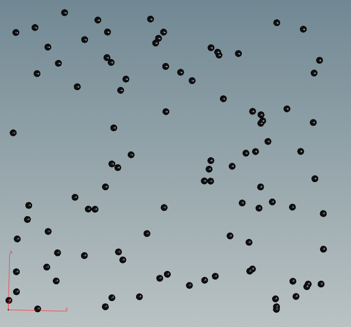
Next we want to illustrate with a single example how to sum over each element of a geometry. Let us assume that we are given a system with random points spread over space. Each point is given a particular mass as a floating point attribute. This could for example model planets in space.

We model them by uniformly randomly distributed points in the $[0,1]^2$ box in the XZ-plane. The number of points is read from an integer parameter in the node interface that we created just like in previous tutorials.
|
1 2 3 4 5 6 7 8 9 10 11 12 13 14 15 16 17 18 19 20 21 |
// create n randomly distributed points. // read how many points from the parameter interface int numOfPoints = int(ch("numOfPoints")); // geometry self reference ( =0 ) int geo = geoself(); // random point creation for( int i = 0; i < numOfPoints; i++){ // random seed int C = 113*numOfPoints; float randx = rand(i*C+1); float randz = rand(i*C+3); // you can also use nrandom() for non-deterministic random numbers // creat point vector Pos = set(randx,0,randz); int vertexid = addpoint(geo,Pos); } |
|
1 2 3 |
// Assign random mass. @P.x serves as a seed. float mass = rand(i@ptnum+@P.x); f@mass=mass; |
Example: total mass
This task is very simple. We run our index from 0 to the (total number of points-1) on each point and sum up the masses we find. This happens in a attribute wrangle running over “detail“.
|
1 2 3 4 5 6 7 8 |
// iterate over each point index and sum up the attributes f@totalMass = 0; for( int i = 0; i < npoints(0); i++){ // read float m = attrib(0,'point','mass',i); // sum f@totalMass += m; } |
Example: center of mass
This task can be done quite similarly by running through every point index again reading the mass “mass” and positions “P“. We then perform a weighted averaging with these values.
|
1 2 3 4 5 6 7 8 9 10 11 12 13 14 |
// read total mass float totalmass = f@totalMass; // iterate over each point index and sum up the attributes v@centerOfMass = set(0,0,0); for( int i = 0; i < npoints(0); i++){ // read attrib vector v = attrib(0,'point','P',i); float m = attrib(0,'point','mass',i); // sum up v@centerOfMass += m*v; } // average v@centerOfMass /= totalmass; |
Note that we set our attribute wrangle node to run only once. You can define this inside the node’s parameter controls by switching to Detail (only once). We store the result in an extra attribute to be able access it later.
If you now look at the geometry spreadsheet of the final node you can see that the total mass is roughly half the number of points and that the center of mass is near (0.5, 0, 0.5). We can expect these results when using uniformly distributed values in the interval [0,1].

Neighbor Operations
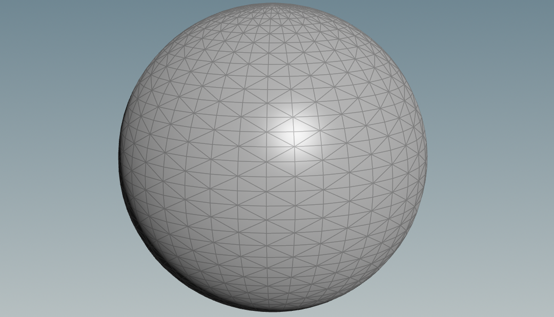
Next we will see how to work with the neighboring points of a single point or with the neighboring faces of a single face. Accessing the right neighbors can be tricky at first. We work with a triangulated version of the surface, and if it is not yet triangulated, we can us a remesh node to archive that.

Let us try it out on a sphere.

Example: edge lengths
Here we want to know the distance between to neighboring points. One could compute the distances between all points to archive that too but that would be computationally too expensive. Instead we can do the following:
Points describe the position of the junctions of our meshes. The GPU however works with vertices and needs 3 vertices to render a triangle even if the points appeared beforehand in another triangle. We have far more vertices than points and we can use this to our advantage. Each vertex is linked to a halfedge (read here to know what halfedges are) from which we can determine the next vertex. We can access the halfedges using vertexhedge(0,@vtnum) and then read the next point in it’s attribute. We do this in a single vertex wrangle node and store the edge lengths multiple times this way.
|
1 2 3 4 5 6 7 8 |
// Run Over: Vertices // grab the length of every half edge int halfEdge = vertexhedge(0,@vtxnum); vector P1 = attrib(0,'point','P',hedge_srcpoint(0,halfEdge)); vector P2 = attrib(0,'point','P',hedge_dstpoint(0,halfEdge)); // and store it as an attribute in each vertex f@edgelength = length(P1-P2); |
Example: triangle areas
Once we know the the edge lengths we can compute the triangle area. Given edge lengths $a,b,c$ we can use the handy Heron’s formula to compute the enclosed area:
$$ p:= \frac{a+b+c}{2} , \ \ \ A=\sqrt{p(p-a)(p-b)(p-c)}$$
This means that we can split this problem into finding the edge lengths first and then using the above formula. We can use the same node as above to compute the edge lengths and then attach another node below to it that computes the area. The primitive wrangle will run on each triangle and extract the edge lengths around it by grabbing any one of the half edges around it and then reading the vertexes through them.
|
1 2 3 4 5 6 7 8 9 10 11 12 13 14 15 16 17 18 19 20 21 22 23 24 25 26 27 28 |
// Run Over: Primitives // an implementation of Herons Formula float HeronFormula(float a; float b ; float c){ // computes the area of a triangle given it's edge lengths float p= 0.5*(a+b+c); return sqrt(p*(p-a)*(p-b)*(p-c)); } // given an id of a triangle, compute it's area float getTriangleArea(int primitiveID){ int geo = 0; // default geometry // grab any one edge around the triangle int halfEdge = primhedge(geo,primitiveID); // read all 3 vertices around the triangle int v1 = hedge_srcvertex(geo,halfEdge); int v2 = hedge_dstvertex(geo,halfEdge); int v3 = hedge_presrcvertex(geo,halfEdge); // extrac all edge lengths from these vertices float a = attrib(geo,'vertex','edgelength',v1); float b = attrib(geo,'vertex','edgelength',v2); float c = attrib(geo,'vertex','edgelength',v3); // apply Heros formula return HeronFormula(a,b,c); } // create an attribute on the triangle with the area f@area = getTriangleArea(@primnum); |
Example: total surface area
This is just like the total mass example above. Instead of summing over the points we now sum over the triangles (primitives) using a attribute wrangle node that runs only once.
|
1 2 3 4 5 6 7 8 9 10 11 |
// Run Over: Detail // iterate over each primitve index and sum up the attributes f@totalArea = 0; int nrOfPrimitives = @numprim; for( int i = 0; i < nrOfPrimitives; i++){ // read float area = attrib(0,'primitive','area',i); // sum v@totalArea += area; } |


Volume Operations
A volume is a 3D grid of values. As such, we would like to know how to access neighbours inside it. Volumes come with their own special kind of attributes, important ones being @resx, @resy, @resz to encode the resolution of the grid.

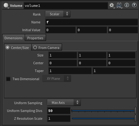
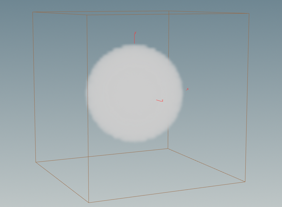
Analogous to the tutorial of the advection, we will create a scalar volume and name its scalar f. We will later blur the function f by its surrounding values. Be sure to set “Uniform sampling Divisions” to be around 50.
Let us make the volume a interesting by editing f inside a volume wrangle node. The next code will define a non-zero constant field inside a sphere.
|
1 2 3 4 5 6 7 8 9 10 11 12 |
// Volume Wrangle // define one field function here // values inside sphere only float r = 0.3; float l = length(@P); // inside sphere if(l<r){@f=1;} else {@f=0;} @f*=10; |
Then inside the repeating loop of the blurring, we need the following code:
|
1 2 3 4 5 6 7 8 9 10 11 12 13 14 15 16 17 18 19 20 21 22 23 24 25 26 27 28 |
// Volume Wrangle // function f blur with uniform weights. // define size of local blurring area int blurResX = 2; int blurResY = 2; int blurResZ = 2; // summ of all values in volume neigbourhood float sum=0; // pick indices around out current index for (int dx=-blurResX; dx<blurResX+1; dx++) { for (int dy=-blurResY; dy<blurResY+1; dy++) { for (int dz=-blurResZ; dz<blurResZ+1; dz++) { // compute neighbour index int jx = (@ix+dx) % @resx; int jy = (@iy+dy) % @resy; int jz = (@iz+dz) % @resz; // add its value to the total sum sum += volumeindex(0,"f",set(jx,jy,jz)); } } } // divide by number of elements in the area float fac = (2*blurResX+1)*(2*blurResY+1)*(2*blurResZ+1); @f =sum/fac; |
@ix, @iy, @iz refer to the index of the piece of volume (the grid box) inside the volume. Using volumeindex(0,”f”,set(jx,jy,jz)) we can then access the volume values by index. The way we perform modular division with % @resx is justified by thinking that the volume is periodically repeating like a torus. Yes, there is a Houdini node that does exactly this job, but writing the code our self is a valuable exercise.
About Begin End Blocks
In case you wondered what the orange net was in the volume blurring: we can place a Block Begin node and a Block End node and have them reference each other to know what operations to repeat on the same geometry over and over again. The orange Net is spanned automatically around the affected area once the two nodes are linked.

To have them reference each other, go to one of the blocks and type in the node reference or select the node manually by clicking on the right of Default Block Path as seen in the gif.