
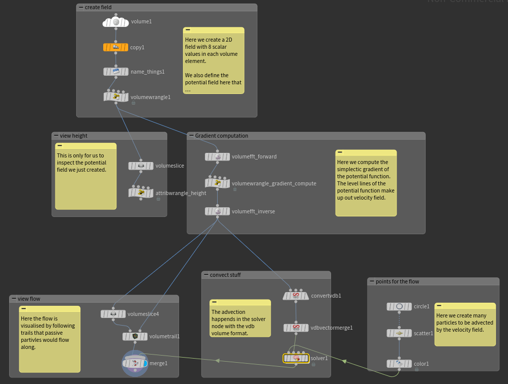
In this tutorial we will work with special nodes in order to visualize the flow of particles inside vector fields. This will be an opportunity to experience the strengths of houdini in action. To accomplish this we will look at many individual tasks that each teach a valuable lesson.

Volumes

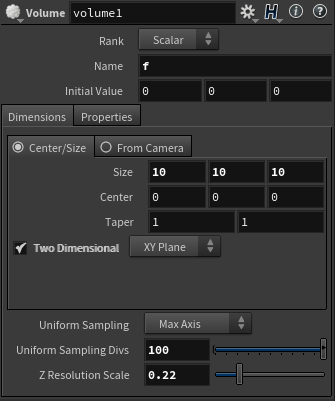
Volumes in houdini represent the segmentation of space into a grid of voxels (like pixels) that each contain some information such as a scalar, a vector etc… . We can also choose 2D volumes which are like grids but will allow us to use Fourier transforms. Place a Volume node and check the Two Dimensional XY plane box, pass on the name f for our scalar values (automatically type float) and adjust the sampling of the volume. Now f is an attribute of the volume ( @f ).
Now we want to have not just one value in each volume element but many. To do this we place a copy and transform node and duplicate the source group @name=f eight times.

To enable us to reference these copies we will name them using a name node. Just go through the numbers and insert each name once.

Now we have access to 8 attributes in each voxel (volume element) of type float. Here we choose these attributes:
- f = real part of potential field
- g = imaginary part of potential field (=0). Important for Fourier transform.
- gradf_x, gradg_x, gradf_y, gradg_y, sgradf_x, sgradf_y = gradient values and simplectic gradient of f and g to later specify.
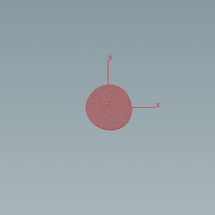
At last we can define the field simply by defining f in the volume wrangler.
|
1 2 3 4 5 6 7 8 |
// define one field function here float x = @P.x; float y = @P.y; // add first field @f= sin(x+1.2*y); // add more fields @f=@f+ cos(sin(x)*.8+cos(y)); @f=@f+ -cos(4*(sin(x)*.8+cos(y))); |
Optional: inspect potential field
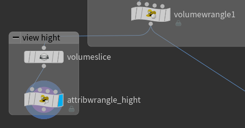
Place a volume slice node to color encode the volume and then transform the height to get a graph like view. The source group of the volume slice must be @name=f.

The attribute wrangler can shift the points along the normal @N and as far as the @density which is an important attribute of volumes.
|
1 2 |
// just to visualize the field as a graph @P+=@density*@N; |
Gradient Computation, Fourier transforms
Next we want to compute the gradient of f. We will archive this with sneaky mathematical tricks who’s explanation would blow up the scope of this course.
We can transform f and g through Fourier transformation back and forth while checking center DC.


The inverse transform carries the source groups:
@name=f @name=g @name=gradf_x @name=gradg_x @name=gradf_y @name=gradg_y @name=sgradf_x @name=sgradf_y
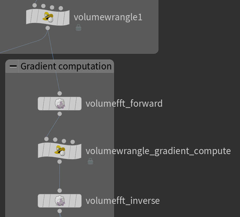
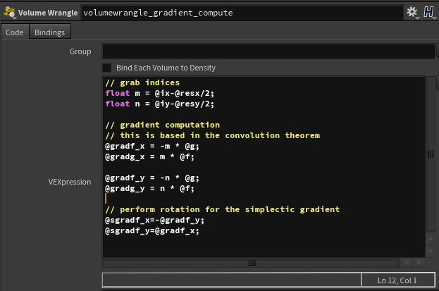
In between the Fourier transformations you can run the following volume wrangler to compute the gradients.
|
1 2 3 4 5 6 7 8 9 10 11 12 13 14 15 |
// grab indices float m = @ix-@resx/2; float n = @iy-@resy/2; // gradient computation // this is based in the convolution theorem @gradf_x = -m * @g; @gradg_x = m * @f; @gradf_y = -n * @g; @gradg_y = n * @f; // perform rotation for the simplectic gradient @sgradf_x=-@gradf_y; @sgradf_y=@gradf_x; |
The Advection of Points
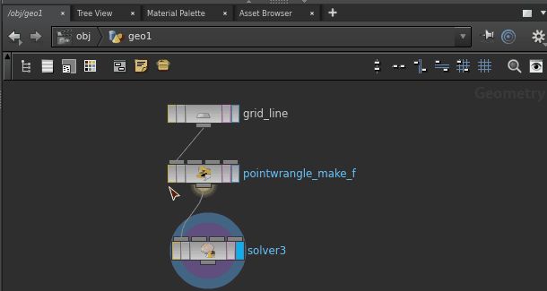
Now we would like to have some points to advect along the simplectic gradient. In order to do that we first need points. We can create a set of points by connecting a circle node with a scatter node. These will be linked to the first input of the solver node.

Before we can advect the flow we need to convert the simplectic gradient volumes into a vdb volumes using the convert VDB node. This is a type of volume used especially for these computations (sparse representation).

We then merge the x and y components into one vector using the VDB Vector merge node.

Next we set up a solver node and dive into it. There we connect the input_2 (our points that will flow) and the previous frame node with an VDB advectpoints node and highlight it.

If we now highlight the solver node we can already see the flow moving when play is pressed.
Remember from the previous tutorial on solver nodes that if you want to see the start before the first advection that you need to uncheck something in the options as seen in the gif below.
Visualizing the Flow
Next we want to take a look at the flow lines. We can archive this by making another volume slice as done and connecting the output of the gradient with a volume trail node.

The volume trail node should should have the simplectic gradients as it’s inputs.

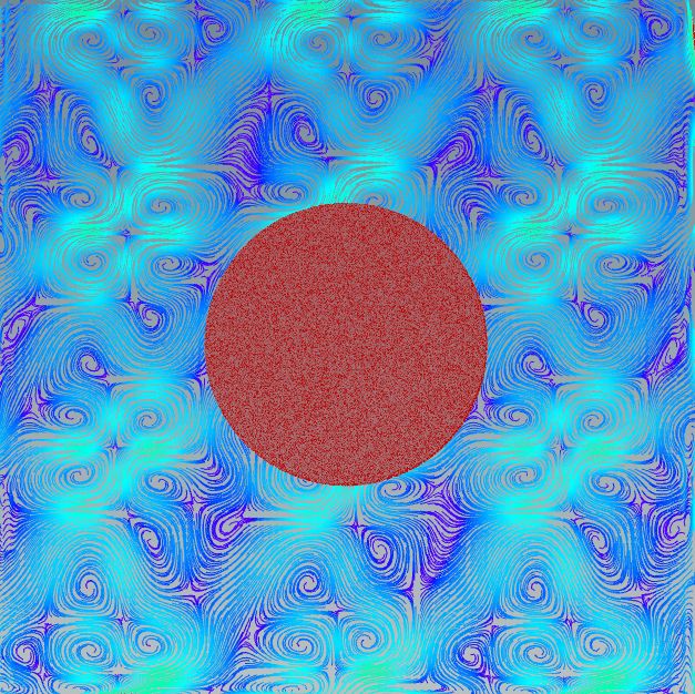
The volume trail itself lets you view the flow lines as seen in the following image.

Results
With a few nodes and very little code we have now archived a functional flow visualization. This is the strength of houdini.
First we show the flow with the flow lines.
And here we show the same flow without the flow lines.

Also keep in mind that a lot of the code that we learned here can be reused. Here we had a constant 2D field but one might as well change the field at every frame for instance to simulate a fluid.
