In this tutorial we will show how to perform more complex tasks using solver nodes.

We will show this using a simple example. Our goal will for now be to implement an iterative method to observe the values of

$$F_n(x,y)=F( F_{n-1}(x))$$

for increasing $n\in\mathbb{N}$ and $F_0(x) = sin(x)$. In other word: applying the $sin(x)$ function repeatedly.

There are a few ways to run iterations in Houdini.  One way is to use “ForLoop” node.  Another way is to turn the “time line” of Houdini into our iteration.  We will use the latter approach.

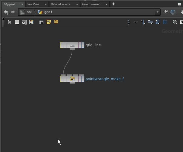
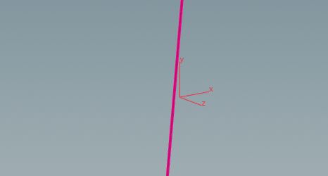
But first lets create a basic line with 100 points and size 3 using a grid node as seen in the image below.

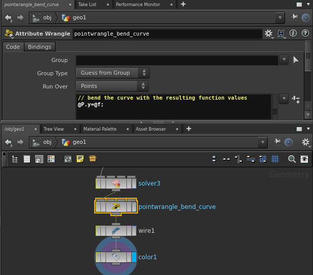
And initialize the attribute @f with another point wrangle node below. “f” refers to the function output.

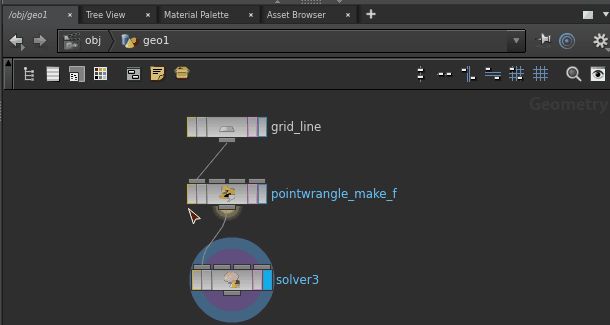
Create a Solver node downstream of the point wrangle node. Dive into this solver node. You will observe a (purple) node labeled “Previous Frame”. As one plays animation, this “Previous Frame” node takes data of the “rendered” node of the previous time frame, which allows us to implement iteration.

Connect the Prev_Frame node to the Input_1 node and attach a point wrangler with the iteration function @f=sin(@f); below and highlight it blue.

One also sees that the path of this solver node is quite complicated: /obj/geo1/solver1/d/s (as seen in the network view top bar). Recall that in /obj there are only limited nodes one could create; that is the land of objects where one creates geometry node or camera or lights. In /obj/geo1 one can create all “SOP nodes” (the nodes we would be working mostly); this is a SOP land or (the land of geometry). You could take a look at /obj/geo1/solver1, it is also a land of SOP. But in /obj/geo1/solver1/d, it is a “DOP land”, the land of dynamics. The nodes you could create in a DOP land is very different from that in SOP land. It contains drivers that are related to the Houdini time line. There is a particular DOP node called “SOP solver” which is a subnetwork in which one has again an SOP land. Before you learn how to take control of DOP network, you don’t need to know any of these details. This solver node already build the DOP part for you, and all you need is to work in /obj/geo1/solver1/d/s, which is an SOP land.

Here is an important trick. Go to /obj/geo1/solver1/d, and on the parameter board, uncheck “Solve Objects on Creation Frame”. If it is checked, then at Frame 1 it would show the result already after one iteration; we uncheck it because usually we want to look at the initial state at Frame 1.

At last we will interprete the output as function values and place them in the @P.y attribute to bend the curve.

So the good thing about solver nodes in this example is that we can compute $F_n$ only using the previous frame and without having to start from $F_0$ every time. One could easily imagine this to play crucial roles when dealing with simulations.

 

Examples of What Solver Nodes Can Do

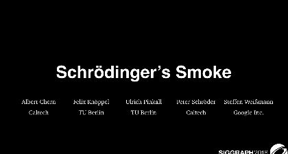
Fluid dynamics is of course a wonderful example of a use solver nodes. The essential computations needed in Schrödinger’s smoke are all created in one solver node.

 

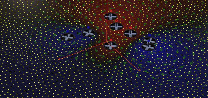
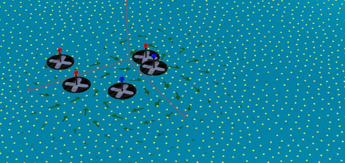
Another example could be vortex motion or particles with gravity interactions. Use the previous frame to compute the forces on each particle and then move them accordingly. To do this, you need a set of points as the input in to the solver node.