
Let us assume that we posses some kind of VEX code definitions for complex functions objects and operators. You can copy and paste the code into a text file that you then name Complex.h.
|
1 2 3 4 5 6 7 8 9 10 11 12 13 14 15 16 17 18 19 20 21 22 23 24 25 26 27 28 29 30 31 32 33 34 35 36 37 38 39 40 41 42 |
#include "math.h" vector2 cmultiply(const vector2 a, b) { return set(a.x * b.x - a.y * b.y , a.x * b.y + a.y * b.x); } void cmultiply(const vector2 z,w; export vector2 a) { float x = z.x * w.x - z.y * w.y; a.y = z.x * w.y + z.y * w.x; a.x = x; } vector2 cinvert(const vector2 a) { float fac = 1/(a.x * a.x + a.y * a.y); return set(fac * a.x , -fac * a.y); } void cinvert(const vector2 a; export vector2 b) { float fac = 1/(a.x * a.x + a.y * a.y); b.x = fac * a.x; b.y = -fac * a.y; } vector2 cpow(const vector2 z; const int n) { vector2 w = {1,0}; for (int j=0; j<abs(n); j++) cmultiply(w,z,w); if (n<0) { cinvert(w,w); } return w; } void cpow(const vector2 z; const int n; export vector2 w) { w.x = 1; w.y = 0; for (int j=0; j<abs(n); j++) cmultiply(w,z,w); if (n<0) cinvert(w,w); } float abs(const vector2 z) { return sqrt(z.x*z.x + z.y*z.y); } |
In the simple curves tutorial we had such a situation where we included code from outside. See the code below to see how it was done in the point wrangle node.
|
1 2 |
#include "math.h" #include "$HIP/include/Complex.h" |
$HIP was used to address the location where the .hip file (or .hipnc) is stored. /include goes into a sub-directory of the current location and /Complex.h located the file with the code. You can think of the #include “filename” command as a copy and paste operator of outside text.

Note: you might have to restart Houdini for it to find the new /include/Complex.h” file if you created it recently.
Try to keep reusable methods neatly organized in directories for usage in other projects.
Using “Export” in Your Custom Code
Normal function definitions normally only allow you to output 1 object of a specific type. Inside function definitions you cannot even have access to attributes that are addressed with @. However, the following trick will make things a lot nicer for us. We will explain how to create multiple outputs of multiple types in a single custom function.
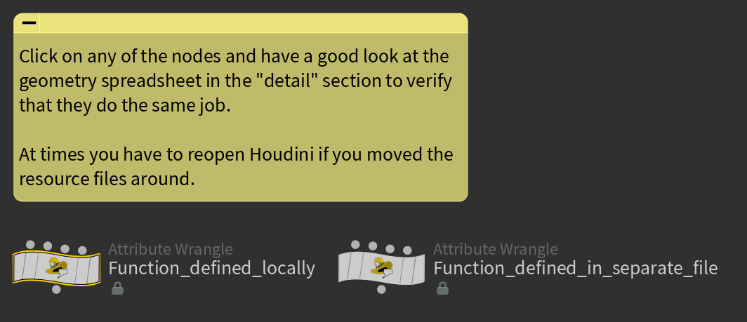
The following two nodes do the exact same job but one of them calls the function form the file while the other one defines it locally inside the node. Defining functions into files is of course the better choice if you reuse a function and if you are done debugging it.
|
1 2 3 4 5 6 7 8 9 10 11 12 13 14 15 16 17 18 19 20 21 22 23 24 25 26 27 28 29 30 31 32 33 34 35 36 37 38 39 40 41 42 43 44 45 46 47 48 49 50 51 52 53 54 |
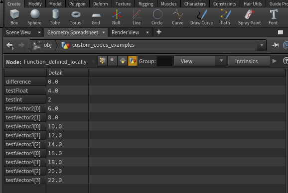
// code of "Function_defined_locally" node // Here we define a function locally just for use inside this node // this test function demonstrates how multiple outputs can be handled at once using export vector testFunction( int myInt; float myFloat; vector2 myVector2; vector myVector3; vector4 myVector4; export int exInt; // exports mean that they will carry to computation outside export float exFloat; export vector2 exVector2; export vector exVector3; export vector4 exVector4; ) { // just scale every single value by two exInt = 2*myInt; exFloat = 2*myFloat; exVector2 = 2*myVector2; exVector3 = 2*myVector3; exVector3 = 2*myVector3; exVector4 = 2*myVector4; // and return the vector3 as an example. You could also make this function void to not return anything return exVector3; } // let us play around with the function // inside this example int testInt; vector test = testFunction( 1, // an int 2.0, // a float set(3.0,4), // a vector2 set(5.0,6.0,7), // a vector3 set(8,9.0,10,11.0), // a vector4 testInt, // reciever of an int f@testFloat, // direct writing into float attrib. u@testVector2, // writing into vector2 attrib. v@testVector3, // writing into vector attrib. p@testVector4); // writing into vector4 attrib. // and copy testInt to attribute to see that this works i@testInt = testInt; // and check the output with the vector 3 f@difference = length(test - v@testVector3); // now check the geometry spreadsheet if everything arrived well |
Notice that our function takes two types of inputs, the regular ones and export inputs. The latter one has the special ability to modify whatever is put into it. This means that you can insert any type of input (int, float, array etc.) and expect the code to write into it. In our example we took the input, scaled it by two and passed it on directly into attributes or another variable through the export slots. Checking the geometry spreadsheet reveals that the output has been successfully passed into the attributes.
Gradient Example
The gradient of a function is a typical example of an operation that you will probably need again and again in the future. This makes it an ideal candidate to go into your beloved “Util.h” file that you can then use in multiple projects in Houdini. The Util.h code can be read at the bottom of this tutorial.
This example can be studied using the supplement material.
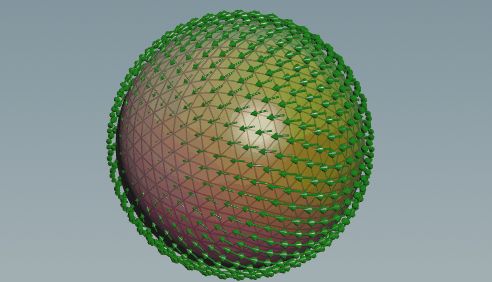
The following example involves the coloring of a sphere (modify @Cd), the creation of an attribute specifically bound to the red part of the color, the computation of the gradient on the triangles for this change in the red color and the averaging of the triangle gradients to the points.

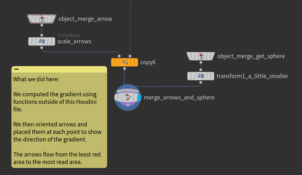
The final results shows the sphere and how the gradient direction of each point on the sphere. Due to our color choice, this gradient field runs from one pole to the opposite.
Here comes the code involved in the making of this gradient:
|
1 2 3 4 5 |
// a point wrangle node // the give_color node // color sphere by normal mapping method @Cd = 0.5*@P+set(.5,.5,.5); |
|
1 2 3 4 5 6 7 8 9 |
// a point wrangle node // the read_red_channel node // delete non red color channels v@Cd.b=0; v@Cd.g=0; // copy read chanel to extra float attribute f@redValue = v@Cd.r; |
|
1 2 3 4 5 6 7 8 9 10 11 12 13 14 |
// a primitive wrangle node // the compute_gradient_of_red_color node // here we import our VEX code functions from outside to use them #include "$HIP/include/Util.h" // use our own gradient computation // as done in discrete exterior calculus gradientField( v@gradRedValue, // grad attrib holder "redValue", // attrib Name to compute gradient from 0, // geo id with the attribute @primnum// id of face ); |
|
1 2 3 4 5 6 7 8 9 10 |
// a point wrangle node // the average_primitives_to_points node // here we import our VEX code functions from outside to use them #include "$HIP/include/Util.h" // averages the attribute of neighbour primitives to the point averagePrimToPoint(v@gradRedValue,@ptnum,"gradRedValue"); // before we had attributes on the triangles, now we have them at points |
|
1 2 3 4 5 6 7 8 9 10 11 12 |
// a point wrangle node // the average_primitives_to_points node #include "$HIP/Include/Util.h" // store rotation at point for visualization vector v = v@gradRedValue; vector dir = v/length(v); vector4 theRotation = orientForCopy(dir,0); setpointattrib(geoself(),"orient",i@ptnum,theRotation); // scale it f@pscale = length(v); |
As promised, here comes the final “Util.h” file as used in this tutorial.
|
1 2 3 4 5 6 7 8 9 10 11 12 13 14 15 16 17 18 19 20 21 22 23 24 25 26 27 28 29 30 31 32 33 34 35 36 37 38 39 40 41 42 43 44 45 46 47 48 49 50 51 52 53 54 55 56 57 58 59 60 61 62 63 64 65 66 67 68 69 70 71 72 73 74 75 76 77 78 79 80 81 82 83 84 85 86 87 88 89 90 91 92 93 94 95 96 97 98 99 100 101 102 103 104 105 106 107 |
#include "math.h" // this file gathers operations that are not specific to one object // this test function demonstrates how multiple outputs can be handled at once using export vector testFunction( int myInt; float myFloat; vector2 myVector2; vector myVector3; vector4 myVector4; export int exInt; // exports mean that they will carry to computation outside export float exFloat; export vector2 exVector2; export vector exVector3; export vector4 exVector4; ) { // just scale every single value by two exInt = 2*myInt; exFloat = 2*myFloat; exVector2 = 2*myVector2; exVector3 = 2*myVector3; exVector3 = 2*myVector3; exVector4 = 2*myVector4; // and return the vector3 as an example. You could also make this function void to not return anything return exVector3; } // return the constant gradient on the faces // needs triangle geometry void gradientField( export vector grad; // grad attrib holder string attribName; // attrib Name to compute gradient from int geo; // geo id with the attribute int primNum // id of face ){ // collect corners int he = primhedge(geo,primNum); vector P1 = attrib(geo,'point','P',hedge_dstpoint(geo,he)); int p1p=hedge_dstpoint(geo,he); he = hedge_next(geo,he); vector P2= attrib(geo,'point','P',hedge_dstpoint(geo,he)); int p2p=hedge_dstpoint(geo,he); he = hedge_next(geo,he); vector P3= attrib(geo,'point','P',hedge_dstpoint(geo,he)); int p3p=hedge_dstpoint(geo,he); // get edges and area vector v1=P3-P2; vector v2=P1-P3; vector v3=P2-P1; vector norm=cross(v1,v2)/length(cross(v1,v2)); float area=length(cross(v1,v2)); // compute gradient grad=1/(2*area)*( attrib(geo,'point',attribName,p1p)*v1 +attrib(geo,'point',attribName,p2p)*v2 +attrib(geo,'point',attribName,p3p)*v3); matrix3 m=ident(); vector axis=norm; float angle=PI/2; rotate(m,angle,axis); grad*=m; } // averages the attribute of neighbour primitives to the point // vector valued void averagePrimToPoint( export vector attrib; // to store result int ptId; // id of point string attributeName // attribute to call for ){ int neighbourPrims[] = pointprims(0, ptId); vector vec = set(0,0,0); foreach (int i ; neighbourPrims){ vec += attrib(0,"primitive",attributeName,i); } attrib = vec/len(neighbourPrims); } // orient an (0,1,0) pointing object to the //new normal and rotate nicley vector4 orientForCopy( vector normal; // final pointing direction float rotation // rotation on that final direction ){ // default vector objectUp = set(0,1,0); // compute quaternions for rotation and orientation seperatly vector4 Qrotate = quaternion(rotation,objectUp); vector4 Qorient = dihedral(objectUp,normal); // collect return qmultiply(Qorient,Qrotate); // combine rotations } |
