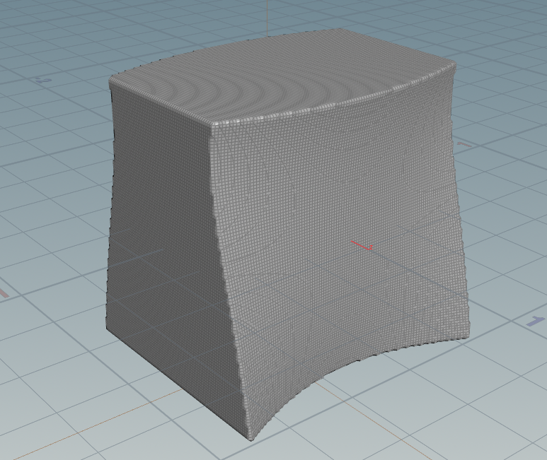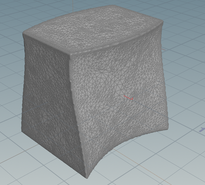
In this tutorial we will start from scratch. We want to know how to create more surfaces.
A natural source of surfaces in space is the constant rank theorem. For maps between Euclidean space it tells us that if \(f\colon U \to \mathbb R^m\), defined on an open \(U\subset\mathbb R^n\), is a smooth map of constant rank \(k\), then \[\mathrm M = f^{-1}(\{q\}),\quad q\in \mathbb R^m\] is an \((n-k)\)-dimensional submanifold. In particular if \(f\colon \mathbb R^3 \supset U \to \mathbb R\) has full rank, then \(\mathrm M\) is a surface in \(\mathbb R^3\).
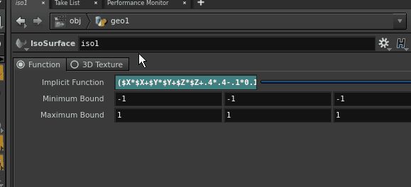
Actually Houdini offers a simple node that allows to create such implicit surfaces. It is called IsoSurface. Here one can specify a function in the coordinates \(\$X\), \(\$Y\) and \(\$Z\) on a volume (3D grid) of a certain size and resolution. Houdini then automatically generates the discrete surface that corresponds to the zero set of the given function.
The results could look like this:
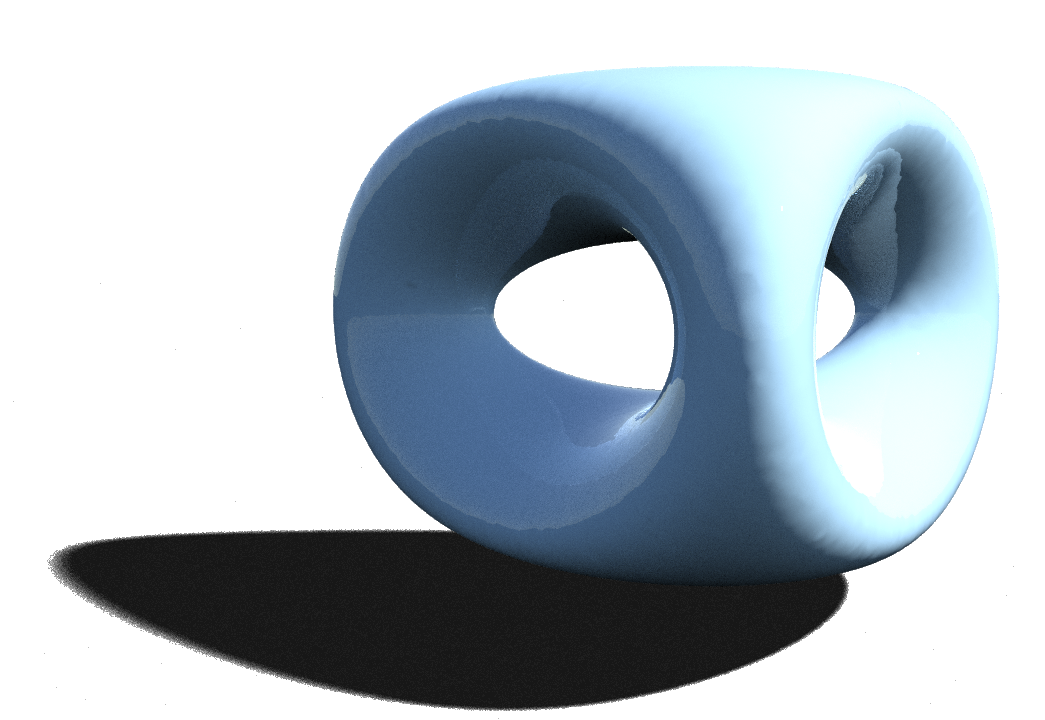
Lets try this out with the following implicit function:($X*$X+$Y*$Y+$Z*$Z+.4*.4-.1*0.1)^2-4*.4*.4*($X*$X+$Y*$Y)
where $X,$Y,$Z refer to the spacial coordinates.
|
1 |
($X*$X+$Y*$Y+$Z*$Z+.4*.4-.1*0.1)^2-4*.4*.4*($X*$X+$Y*$Y) |
Since the values in the volume are interpolated from the values at the points, the resolution of the grid has strong influence on the quality of the result.
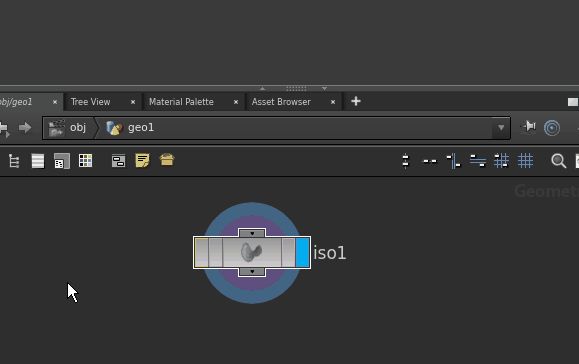
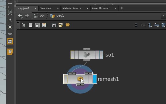
If necessary the extracted discrete surface can be post-processed with a remesh node to obtain a triangulation.
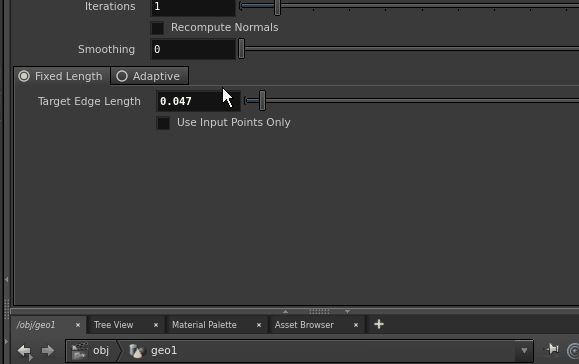
The remesh node can also be manipulated to make the mesh finer.
If for some reason the computations take too long, you can often cancel the computation by hitting the ESC key. Look at the message at the bottom left of the Houdini window to see what is currently computed.
Volumes and Conversion
Lets look how we can use a volume to create an implicit surface.
Volumes in Houdini represent the segmentation of space into a grid of voxels (like pixels) that each contain some information such as a scalar. We we pick a volume of type scalar and name that scalar f we end up having a float type attribute in each voxel. Don’t forget to adapt the resolution of the voxel grid.
Next we are going to give each voxel a new value for f. We do that using a volume wrangle node with the following code:
|
1 2 3 4 5 6 7 8 9 |
float x=@P.x; float y=@P.y; float z=@P.z; float r=0.1; // define some arbitrary function float a=2*y*(y*y-3*x*x)*(1-z*z); float b = pow(x*x+y*y,2); float c =-(9*z*z-1)*(1-z*z); @f= a + b + c -r*r; |
We then link the output to a convertvolume node which does pretty much just what our isosurface node did in the first place but in a more generalized setting. Afterwards we apply another remesh node just to down sample the resolution to relax our computer.
