Let $\gamma_1,\ldots,\gamma_n\in \mathbb{R}^3$ be a regular discrete space curve. We are looking for another discrete space curve $\tilde{\gamma}$ that satisfies the first two conditions we had in the planar case: The distance between corresponding points $|\tilde{\gamma}_j-\gamma_j|$ is a constant $\ell$ and corresponding edges of $\gamma$ and $\tilde{\gamma}$ have the same length. Then (with a notation as in the previous post) we see that compared two the planar case we have a whole one-parameter family of possible choices for $S_{j+1}$: The vector $S_{j+1}$ can be the result of rotating $S_j$ around $\ell S_j + v_j T_j$ by any chosen angle.

One can imagine to start with a parallelogram with sides $v_j T_j$ and $\ell S_j$. The parallelogram is then folded around the diagonal whose direction is $\ell S_j-v_jT_j$.

Folding by 180 degrees corresponds to the Darboux-transformations we studied in the two-dimensional setting. It is given by the map

\[y\mapsto (\ell S_j-v_jT_j)y(\ell S_j-v_jT_j)^{-1}.\]

Any other folding angle (except for angle zero that would leave us with the parallelogram) can be realized as

\[y \mapsto qyq^{-1}\]

with $q$ of the form

\[q=r+\ell S_j-v_jT_j.\]

Here $r$ is an arbitrary real number. This leads to

\[S_{j+1}=(r+\ell S_j-v_jT_j)S_j(r+\ell S_j-v_jT_j)^{-1}\].

Definition: A discrete space curve $\tilde{\gamma}$ is called a Darboux transform of $\gamma$ with rod length $\ell$ and twist $r$ if

\[\gamma_j=\gamma_j+\ell S_j\]

and $S_1,\ldots, S_n$ satisfy the above equation.

Let us omit the subscript $j$ and use a subscript “+” instead of $j+1$. Combining then in the above formula the $S$ in the middle with the left bracket we see that the map $S\mapsto S_+$ is fractional linear:

\[S_+=((r -v T) S-\ell)((r -vT)+\ell S)^{-1}.\]

To investigate this map further we write $S$ as the stereographic projection with center $-T$ of some point $Z\in \mathbb{R}^3$ orthogonal to $T$:

\begin{align*} S &=(1-ZT)T(1-ZT)^{-1} \\\\ &=(T+Z)(1-ZT)^{-1} \\\\ &= T(1-ZT)(1+ZT)^{-1}.\end{align*}

The first line shows that $S\in S^2$ for $Z\perp T$. The second line shows that $Z\mapsto S$ is fractional linear. The last line shows that $S=Z$ in case $|Z|=1$. Let us plug this into the last formula for $S_+$:

\begin{align*}S_+&= ((r-vT)(T+Z)-\ell (1-ZT)((r-vT)(1-ZT)+\ell(T+Z))^{-1} \\\\ &=(((v-\ell)+rT)+(r-(v+\ell)T)Z)((r+(\ell-v)T)+((\ell+v)+rT)Z)^{-1} \\\\ &= \left(T+Z\frac{(\ell+v)-rT}{(\ell-v)-rT}\right)\left(1+TZ\frac{(\ell+v)-rT}{(\ell-v)-rT}\right)^{-1}.\end{align*}

Here the fractional notation is justified because the quaternions involved all commute. Thus in terms of the sterographic coordinate $Z$ the transition from $S$ to $S_+$ is just multiplication

\[Z+=MZ=Z\overline{M}\]

by a quaternion

\[M = \frac{(\ell+v)+rT}{(\ell-v)+rT}.\]

In the case $r=0$ this is in perfect accordance with the results of an earlier post.

Let us first look at the smooth case. Let \(\gamma\colon I\to \mathbb{R}^3\) be an arc length parameterized smooth curve with tangent vector \(T:=\gamma^\prime\).

An adapted frame is then a smooth map \(\sigma\colon I\to SO(3)\) such that \(\sigma e_1 = T\). We denote the second and the third column of \(\sigma\) by \(N\) and \(B\)\[\sigma= (T,N,B).\]The fields \(N\) and \(B\) are normal vector fields. Clearly \(B=T \times N\).

Let us take the derivative of \(\sigma\). Since the vectors \(T,N,B\) are normalized we find that\[\sigma^\prime=\sigma \mathcal{U},\]where\[\mathcal{U}=\begin{pmatrix}0 & \kappa_1 & \kappa_2 \\ -\kappa_1 & 0 & -\tau \\ -\kappa_2 & \tau & 0 \end{pmatrix}.\]

If \(N\) is parallel along \(\gamma\), i.e. the derivative has only a tangential component \(N^\prime= \kappa_1 T\), then so is \(B\), and \(\tau\) vanishes:\[\mathcal{U}=\begin{pmatrix}0 & \kappa_1 & \kappa_2 \\ -\kappa_1 & 0 & 0 \\ -\kappa_2 & 0 & 0 \end{pmatrix}.\]Such a frame is called a parallel frame. We have seen in the lecture that parallel frames always exist.

If \(\sigma=(T,N,B)\) is a parallel frame and \(\alpha\in\mathbb{R}\), then we define a new frame \(\sigma_\alpha= (T,N_\alpha,B_\alpha)\) with \[N_\alpha = \cos\alpha\, N+ \sin\alpha\, B,\quad B_\alpha=-\sin\alpha\, N+ \cos\alpha\, B.\]This frame is parallel again.

The point now is that, up to Euclidean motion, \(\gamma\) is determined by \(\mathcal{U}\). We can just solve for \(\sigma\) and obtain \(T\) as its first column. The curve is then reconstructed by integrating \(T\).

The term spinning refers then to the following procedure. We start with a curve \(\gamma\) and a parallel frame \(\sigma\). This gives us \(\mathcal{U}\) with \(\kappa_1\) and \(\kappa_2\). Now we define \(\mathcal{U}_\lambda\) for \(\lambda\in\mathbb{R}\) as follows\[\mathcal{U}_\lambda=\begin{pmatrix}0 & \kappa_1 & \kappa_2 \\ -\kappa_1 & 0 & -\lambda \\ -\kappa_2 & \lambda & 0 \end{pmatrix}.\]This determines a new curve \(\gamma_\lambda\). This family of curves is called the associated family.

  

Our plan is to spin discrete space curves. So let \(\gamma=(\gamma_0,\dots,\gamma_n)\) be a discrete space curve. Thinking of linear interpolation one finds the best place to locate an adapted frame is on the edges. Here it is clear what the tangent \(T_i\) shall be\[\gamma_i^\prime:=\gamma_{i+1}-\gamma_i= \ell_i T_i.\]

Since the tangent on each edge is constant, we can put just a constant frame on each edge, i.e. for each edge we get \(\sigma_i\) such that \(\sigma_i e_1= T_i\). Only at vertices the frame field has to jump.

We define a discrete adapted frame as a collection of \(SO(3)\)-matrices \(\sigma_i\) such that \(\sigma_i e_1= T_i\).

The jumps over the vertices are again given by \(SO(3)\)-matrices \(\mathcal{U}_i\), which we will call transport matrices. Quiet analogue to the smooth we have\[\sigma_i= \sigma_{i-1} \mathcal{U}_i.\]

As in the smooth world the transport matrices determine the adapted frame. If a initial value \(\sigma_0\) is given then \(\sigma_i\) is given by\[\sigma_i=\sigma_0\mathcal{U}_1 \cdots\mathcal{U}_i.\]

The corresponding curve is then reconstructed by integration of \(T= \sigma e_1\). So we get for \(\gamma_0\in \mathbb{R}^3\) and \(\sigma_0\):\[ \gamma_{k+1} = \gamma_0 + \sigma_0 \bigl(\sum_{i=0}^k \ell_i\mathcal{U}_1 \cdots\mathcal{U}_i\bigr)e_1.\]

Again we find special transport matrices, namely these which change the frame as minimal as possible, i.e. if \(T_{i-1}\) and \(T_i\) are parallel then \(\mathcal{U}_i=Id\) and else \(\mathcal{U}_i\) rotates \(\sigma_{i-1}\) around \(T_{i-1}\times T_i\). These transport matrices we will denote by parallel transport. They come directly with the geometry of the curve.

A frame with such transport matrices is called a discrete parallel frame. Each discrete curve admits a parallel frame.

Now let \(\gamma\) be a discrete space curve with a parallel frame \(\sigma=(T,N,B)\). Then this defines complex numbers \(q\) at the vertices in the following way: Consider the vertex \(\gamma_{i+1}\). The plane \(\mathcal{N}_{i}\) spanned by the vectors \(N_{i},B_{i}\) can be considered as complex line with rotation given by 90-degree-rotation around \(T_{i}\) which we will denote by \(J\), i.e. \(JX=T_i\times X\). The next tangent vector \(T_{i+1}\) lies on the unit sphere with the point \(-T_{i}\) removed.

If we perform stereographic projection with respect to the north pole \(-T_{i}\), then the tangent vector \(T_{i+1}\) is mapped to \(\mathcal{N}_i\) and hence defines a complex number \[q_{i+1}=\kappa_1\, N_i + \kappa_2 B_i=(\kappa_1 + \kappa_2 J) N_i.\] This can be interpreted as discrete complex curvature.

If the tangents are linearly dependent then \(q=0\). If they are not they span a plane. We slice the sphere by this plane and find that the magnitude of \(q\) is given by\[|q|= \tan(\tfrac{\alpha}{2}),\]where \(\alpha\) is the angle between \(T_i\) and \(T_{i+1}\).

In general frames can have torsion. While the curvature is located at the vertices, we define the torsion on the edges. Let \(\sigma\) be an arbitrary frame. Imagine the frames located at the start of the edges. We want to know how much it rotates around the edge from the beginning to the end. To get the rotation angle we use the parallel transport to pull the frame on the next edge back to the end of the current. I.e. we have \(\sigma_i\) and \(\sigma_{i+1}\mathcal{U}_{i+1}^{-1}\), both adapted to the i-th edge. They differ by a rotation around \(T_i\). If \(\alpha\) is the angle of the rotation, then the torsion \(\tau_i\) is given by \[\alpha= \tau_i \ell_i.\]

To go further, we change to quaternionic frames in which the transports takes a much simpler form. Therefore we identify \(\mathbb{R}^3\) with the imaginary quaternions, i.e.\[x_1e_1+x_2e_2+x_3e_3 \longleftrightarrow x_1\mathbf{i}+ x_2\mathbf{j}+x_3\mathbf{k}.\]With this identification a rotation around an axis given by a vector \(X\) with \(|X|=1\) by an angle \(\alpha\) takes the form\[P\mapsto X_\alpha PX_\alpha^{-1},\]where \[X_\alpha=\cos(\alpha/2)\mathbf{1} +\sin(\alpha/2)X.\]

So we can encode the frame equations by quaternions by considering \(\phi_i\) such that\[T_i = \phi_i\, \mathbf{i}\,\phi_i^{-1},\quad N_i = \phi_i\, \mathbf{j}\,\phi_i^{-1},\quad B_i = \phi_i\, \mathbf{k}\,\phi_i^{-1}.\]That is \(\phi\) rotates the standard basis to the basis given by the frame \(\sigma_i\). By the equations above \(\phi_i\) is determined up to a non-zero scale factor. As before the frames \(\phi_i\) are related by transports, i.e.\[\phi_{i}=\phi_{i-1}\mathcal{V}_i.\]

The reconstruction formula for the corresponding curve takes a quite similar form\[\gamma_{k+1}= \gamma_0 + \phi_0\bigl( \sum_{i=0}^{k}\ell_i (\mathcal{V}_1\cdots \mathcal{V}_i )\,\mathbf{i}\, (\mathcal{V}_1\cdots \mathcal{V}_i)^{-1}\bigr)\phi_0^{-1}.\]

Once we know the \(q\) the parallel transport takes an amazingly simple for in the quaternionic setting. It is given by \[\mathcal{V}_i = \mathbf{1}+ \mathbf{i}q\mathbf{j}= \mathbf{1}+ q\mathbf{k}= \mathbf{1} -\operatorname{Im}(q)\mathbf{j}+\operatorname{Re}(q)\mathbf{k}.\]

This is due to the fact that \(-\operatorname{Im}(q)\mathbf{j}+\operatorname{Re}(q)\mathbf{k}\) are the coordinates (wrt. \(\phi_{i-1}\)) of the rotation axis prescribed by parallel transport and \(|q|=\tan(\alpha/2)\), where \(\alpha\) is the rotation angle.

The rotation around the tangent takes the simple form \(\mathcal{T}_i^\alpha=\cos(\alpha\ell_i)\mathbf{1}+\sin(\alpha\ell_i)\mathbf{i}\). Hence we can spin the curve in the following way:

1. Take a parallel frame and calculate the corresponding \(q\)’s.
2. Define for \(\lambda\in \mathbb{R}\) a new parallel transport by \(\mathcal{V}^\lambda_i=\mathcal{T}^\lambda_{i-1}\mathcal{V}_i\).
3. Reconstruct the curve corresponding the \(\mathcal{V}^\alpha_i\).

 

Homework (due date 27 June): Your task is to implement the spinning procedure, i.e. write a plugin the constructs for a given \(\lambda\in\mathbb{R}\) the curve corresponding to the transports \(\mathcal{V}^\lambda_i\) as define above and adds it to the scene. The initial values should be chosen suitably.

As in the last post let $\gamma$ be a discrete curve in the $\mathbb{C}$ and $\tilde{\gamma}= \gamma+ \ell S$ be a Darboux transformation. Denote by $\alpha_j$ and $\beta_j$ the angles from the edges $T_J$ of $\gamma$ to the rod directions $S_j$ and $S_{j+1} respectively. Then

\begin{align*}S_j &= e^{i \alpha_j} T_j \\\\ S_{j+1}&= e^{i \beta_j} T_j.\end{align*}

We know that $S$ satisfies

\[ S_{j+1}=\frac{\ell S_j- v_j T_j}{\ell-v_j \bar{T}_j S_j}.\]

This yields

\[ e^{i\beta_j}=\frac{\ell e^{i\alpha_j}- v_j}{\ell-v_j e^{i\alpha_j}}.\]

Using the formula

\[e^{i\alpha}=\frac{1+it}{1-it}\]

where

\[t:=\tan \frac{\alpha}{2}\]

we then have

\begin{align*} e^{i\beta_j}&=\left(\ell \frac{1+it_j}{1-it_j}- v_j \right) \left(\ell-v_j \frac{1+it_j}{1-it_j} \right)^{-1} \\\\ &=\left(\frac{(\ell -v_j)+(\ell +v_j)it_j}{1-it_j}\right) \left( \frac{(\ell-v_j )-(\ell+v_j )it_j}{1-it_j} \right)^{-1} \\\\ &= \frac{1+i \mu_j t_j}{1-i \mu_j t_j} \,.\end{align*}

where

\[ \mu_j= \frac{\ell+v_j}{\ell-v_j}.\]

From this we conclude

\[\tan \frac{\beta_j}{2}=\mu_j \tan \frac{\alpha_j}{2}.\]

With the notation

\begin{align*}t_j&:=\tan \frac{\alpha_j}{2}\\\\ \tau_j&:=\tan \frac{\kappa_j}{2}\end{align*}

we obtain

\begin{align*}\tau_j&=\tan \frac{\beta_{j-1}-\alpha_j}{2}\\\\ &= \frac{\mu_{j-1} t_{j-1}-t_j}{1+\mu_{j-1} t_{j-1} t_j}.\end{align*}

The corresponding quantities for the Darboux transform $\tilde{\gamma}$ are

\begin{align*}\tilde{\alpha}_j &=\pi-\beta_j \\\\ \tilde{\beta}_j &= \pi- \alpha_j \\\\ \tilde{\tau}_j&=\tan \frac{\beta_j-\alpha_{j-1}}{2}\\\\ &= \frac{\mu_j t_j-t_{j-1}}{1+\mu_j t_j t_{j-1}}.\end{align*}

Note that we arrive at $\tilde{\tau}_j$ starting from $\tau_j$ if we interchange the roles of $t_{j-1}$ and $t_j$ and replace $\mu_{j-1}$ by $\mu_j$. If we apply this rule to

\begin{align*}1+\tau_j^2 &= \frac{(1+2\mu_{j-1} t_{j-1} t_j +\mu_{j-1}^2 t_{j-1}^2 t_j^2) + (t_j^2 -2 \mu_{j-1} t_{j-1} t_j +\mu_{j-1}^2 t_{j-1}^2)}{(1+\mu_{j-1} t_{j-1} t_j)^2} \\\\ &= \frac{(1+t_j^2)(1+\mu_{j-1}^2 t_{j-1}^2)}{(1+\mu_{j-1} t_{j-1} t_j)^2} \end{align*}

we obtain

\[1+\tilde{\tau}_j^2=\frac{(1+t_{j-1}^2)(1+\mu_j^2 t_j^2)}{(1+\mu_j t_j t_{j-1})^2}\]

Now the following is easy to prove:

Theorem: If $\gamma$ is a closed polygon in $\mathbb{R}^2$ with equal edge lengths and $\tilde{\gamma}$ is a closed Darboux transform of $\gamma$ then

\[\prod_{j=1}^n (1+\tau^2) = \prod_{j=1}^n (1+\tilde{\tau}^2).\]

We can interpret this as follows: The bending energy

\[\sum_{j=1}^n \log (1+\tau_j^2)=-\sum_{j=1}^n \log (1+\cos \kappa_j)\]

is the same for $\gamma$ and $\tilde{\gamma}$.

As we saw in the  lecture, we can parametrize the moduli space of discrete closed plane curves by angles and edge lengths, which encode how the tangent is moving along the curve. More explicit: up to rigid motion each discrete curve with \(n\) vertices and tangent winding number \(m\) is represented by a point in a submanifold \(\mathcal{M}_0\) of \((-\pi,\pi)^{n}\times (0,\infty)^{n}\), which is given by the zero set of the map \[ F:(-\pi,\pi)^{n}\times (0,\infty)^{n} \to \mathbb{R}^3 = \mathbb{R}\times \mathbb{C}\\\\ F(\ell,\kappa)=\left(\begin{array}{c} \kappa_1+\ldots +\kappa_n -2 \pi m \\  \ell_1 e^{i\alpha_1}+\ldots +\ell_{n}\, e^{i\alpha_{n}}\end{array}\right),\] where \[\alpha_j= \kappa_1+\ldots+\kappa_j.\]

In general, each function defined on \(\mathcal{M}\) splits the space into components. E.g. think  of a height function of an embedded surface.

If the map is ‘nice’ enough, i.e. in our case smooth and of constant rank, then the level sets are submanifold. Moreover \(\mathcal{M}_0\) is the intersection of the submanifolds \(\mathcal{M}_1\) and \(\mathcal{M}_2\), which are given as zeros sets of the functions\[F_1(\ell,\kappa)=\kappa_1+\ldots +\kappa_n -2 \pi m, \quad F_2(\ell,\kappa)=\ell_1 e^{i\alpha_1}+\ldots +\ell_{n}\, e^{i\alpha_{n}}.\]

Now, we have given \(\mathcal{M}_0\) which parameterizes discrete closed plane curves. But what does the ambient space correspond to?

It is important to note that a closed curve is in fact rather a periodic sequence of points than just \(n\) points. With this in mind, let us assign to each point in \((-\pi,\pi)^{n}\times (0,\infty)^{n}\) periodic sequences, denoted again by \(\kappa\) and \(\ell\), to which corresponds a discrete curve \(\gamma \colon \mathbb{Z}\to \mathbb{C}\). The curve \(\gamma\) is obtain by ‘integration’, i.e. e.g. for positive \(k\) we have\[\gamma_{k+1}=\sum_{j=1}^k \ell_j e^{i\alpha_j}.\]

Now we can directly look at the effect of dropping conditions: Let us start outgoing from the case that \(\kappa,\ell\) lies on \(\mathcal{M}_0\), i.e. we have a discrete closed plane curve as shown below.

If we drop the second condition we just stay on \(\mathcal{M}_1\), i.e. the curves do not have to close up but the tangent winding number is still restricted to \(2\pi m\), such curves are know as curves with translational period. Examples are shown below.

These curves can also regarded as closed curves on a cylider.

Our task is now to navigate on the submanifold \(\mathcal{M_0}\), i.e. given a vector field \(X\) on \(\mathcal{M_0}\) and a point \(p \in\mathcal{M_0}\), then move along the integral curve of \(X\) starting at \(p\).

In our setup we are surrounded by a Euclidean space that means that tangent vector fields are just maps into \(\mathbb{R}^{2n}\). First, let us ignore all conditions for a moment. Then we can just use the Euler method to follow the vector field, i.e. we just go a bit in the direction of the vector field: If at time \(t\) we are at the position \(p(t)\), then \[ p(t+\varepsilon)= p(t)+\varepsilon X(p(t)),\] is the position at time \(t+\varepsilon\). Since this shall correspond to a discrete curve that was obtained by regular homotopy we have to ensure that we don’t leave the open subset \((-\pi,\pi)^{n}\times (0,\infty)^{n}\). But that’s easy.

It is also easy to stay in \(\mathcal{M}_1\) as it consists of open subsets of affine vector spaces, i.e. all one has to do is to project the given vector field \(X\) to the tangent space of \(\mathcal{M}_1\). If \(X^\top\) denotes the projection, the corresponding line \(p+\operatorname{span}\{X^\top(p)\}\) is then already contained in the affine vector space. Again all we have to ensure is that the point does not leave an open set.

The situation changes if we start at a closed curve \(p(t)\) and want to stay closed. First, the vector field then has to be tangential to \(\mathcal{M}_0\), i.e. we have to eliminate the normal components. Second, even if the field is tangential, we will leave \(\mathcal{M_0}\) Immediately if we move along a line. Our strategy will be to fix this by projecting back to \(\mathcal{M_0}\) after each Euler step.

Let us focus on the situation that all lengths shall stay fixed during the flow as it was presented in the lecture, i.e. all components of the vector field that correspond to lengths are just zero:\[X(p)=(X_1(p),\dots,X_{n}(p),0,\dots,0).\]

The normal space to \(\mathcal{M}_0\) at a point \(p=(\kappa_1,…,\kappa_{n},\ell_0,…,\ell_{n}) \in \mathcal{M}_0\) was spanned by \[V_0=(1,\dots,1,0,\dots,0)\] and the vertex coordinates of a curve \(\gamma\) corresponding to the point \(p\) \[ V_1=(x_1,\dots,x_j,0,\dots,0),\\ V_2=(y_1,\dots,y_j,0,\dots,0),\] where the \(x_j\) and \(y_j\) denotes the real and imaginary part of \(\gamma_j\) resp., i.e. \(\gamma_j=x_j+iy_j\).

We apply the Gram-Schmidt process starting with \(V_0\) and obtain an orthonormal basis \(N_0,N_1,N_2\) of the normal space of \(\mathcal{M}_0\). The projection of \(X\) on its tangential part \(X^T\) then takes the simple form\[X^\top=X-\sum_{j=0}^2\langle X,N_j\rangle N_j.\]

We perform the Euler step with respect to the field \(X^\top\) and obtain a new point \(\tilde p=(\tilde\kappa,\ell)\) which a priori not yields a closed curve. Now we have to get back to \(\mathcal{M}_0\), i.e. we have to change the \(\tilde\kappa\) slightly so that \(F(\tilde\kappa,\ell)=0\). Hence we have to search for a zero of a non-linear function in an \(n\)-dimensional space, which in general is slow and the speed moreover depends on the number of vertices.

We reduce this problem, as proposed, to a \(2\)-dimensional one by projecting \(\tilde p\) back along the normal space at the previous point \(p\):\[f(\lambda_1,\lambda_2)=F(\tilde\kappa+\lambda_1N_1+\lambda_2 N_2,\ell)=0.\]

This we solve by applying the Newton method and obtain a new closed curve.

Homework (due date 6 June): Your task is to implement the gradient flow of the bending energy on closed curves. In the repository you find under de.jtem.discreteCurves.tutorial a class called GradientFlowPlugin which provides a basic environment to start with. It shows the gradient flow of the bending energy\[E(\kappa,\ell)= \tfrac{1}{2}\sum_{j=1}^{n} \kappa_j^2.\] without any constraints, i.e. closed curves immediately open up and are deformed into straight lines.

Copy the GradientFlowPlugin into your project.

Your task is now to modify the flow so that closed curves stay closed, i.e. you have the following things to do:

1. Project the gradient of the bending energy to the tangent space of \(\mathcal{M}_0\) to obtain a vector field \(X\) which is tangential.
2. Implement the projection back to \(\mathcal{M}_0\) after the Euler step.

The Euler step just stays as it is. For the second item you can use the Newton method that is implemented in the jtem project numericalMethods (explicitly in de.jtem.numericalMethods.calculus.rootFinding).

Hint: Even if it is not an example for the usage of the Newton-class it may be helpful to look into ExampleNewtonRaphson, which you find at the same place.

In this post we will work with a fixed sequence of lengths  $\ell_1,\dots,\ell_n>0$. This means we imagine polygons as composed of rigid edges connected by flexible joints at the vertices. Denote by $\mathcal{M}_m$ the space of curvature functions $\kappa=(\kappa_1,\ldots,\kappa_n)$ that correspond to closed regular polygons with $n$ vertices and tangent winding number $m$.  We can conveniently describe $\mathcal{M}_m$ as the zero set of the function

\begin{align*}\qquad F:(-\pi,\pi)^n &\to \mathbb{R}^3 = \mathbb{R}\times \mathbb{C}\\\\ F(\kappa_1,\ldots,\kappa_n)&=\left(\begin{array}{c} \kappa_1+\ldots +\kappa_n -2 \pi n \\  \ell_0 e^{i\alpha_0}+\ldots +\ell_{n-1}\, e^{i\alpha_{n-1}}\end{array}\right).\end{align*}

By the above calculation the derivative of $F$ is given as

\[F'(\kappa_1,\ldots,\kappa_n)\left(\begin{array}{c}\dot{\kappa}_1\\ \vdots \\ \dot{\kappa}_n\end{array}\right)=\left(\begin{array}{c} \dot{\kappa}_1+\ldots +\dot{\kappa}_n \\ \dot{\kappa}_1 \gamma_1+\ldots + \dot{\kappa}_n \gamma_n \end{array}\right).\]

Theorem: The rank of $F’$ is three at all points of $\mathcal{M}_m$. Therefore, by the implicit function theorem, $\mathcal{M}_m$ is a smooth manifold.

Proof: At a point $(\kappa_1,\ldots,\kappa_n)$ where the columns of $dF(\kappa_1,\ldots,\kappa_n)$ were linearly dependent we would have $a,b,c\in \mathbb{R}$ such that

\[a \mbox{Re}(\gamma_j)+b \mbox{Im}(\gamma_j)+c=0\]

for all $j$. But this means that the whole polygon lies on a straight line, which is impossible for a regular polygon.

$\square$

Suppose we have a vector field tangent to $\mathcal{M}_m$ that we want to follow numerically. This means that for any $\kappa=(\kappa_1,\ldots,\kappa_n)\in \mathcal{M}_m$  we are given a certain tangent vector

\[X_\kappa \in T_\kappa \mathcal{M}_m=\mbox{ker}F'(\kappa).\]

We want to find curves $t\mapsto \eta(t)\in \mathcal{M}_m$ that satisfy for all $t$

\[\dot{\eta}(t)=X_\eta(t).\]

If we already have constructed $\kappa=\eta(t)$ we might attempt to find $\eta(t+\epsilon)$ as

\[\tilde{\kappa}=\kappa+\epsilon \dot{\kappa}\]

where $\dot{\kappa}=X_{\kappa(t)}$. Since $\dot{\kappa}$ lies in the kernel of $F'(\kappa)$ the condition

\[\tilde{\kappa}_1+\ldots+\tilde{\kappa}_n=2\pi m\]

will be satisfied. The second condition

\[\ell_0 e^{i\tilde{\alpha}_0}+\ldots +\ell_{n-1} \,e^{i\tilde{\alpha}_{n-1}}\]

however is non-linear and so we cannot be sure that $\tilde{\kappa}$ corresponds to a closed regular polygon. We first have to project $\tilde{\kappa}$ back to $\mathcal{M}_m$.

To this end we add to $\tilde{\kappa}$ an element of $(T_\kappa\mathcal{M}_m)^\perp$, the normal space to $\mathcal{M}_m$ at the point $\kappa$. This space is spanned by

\begin{align*}N_0&=(1,\ldots,1)\\\\ N_1&=(x_1,\ldots,x_n) \\\\ N_2 &=(y_1,\ldots,y_n)\end{align*}

Here $\gamma_j=x_j+iy_j$ and we assume that a translation has been applied to $\gamma$ in order to achieve

\[\gamma_1+\ldots,+\gamma_n=0.\]

Since the condition $\tilde{\kappa}_1+\ldots+\tilde{\kappa}_n=2\pi m$ already has been dealt with there is no need to work with $N_1$. We therefore are looking for $\lambda_1,\lambda_2 \in \mathbb{R}$ such that

\[f(\lambda_1,\lambda_2)=(0,0).\]

Here

\[f(\lambda_1,\lambda_2)=G(\kappa+\lambda_1 N_1 + \lambda_2 N_2)\]

where

\[G(\hat{\kappa}):=\ell_1e^{i\hat{\alpha}_1}+\ldots+\ell_{n-1}e^{i\hat{\alpha}_{n-1}}\,.\]

Thus we are left with the problem of finding a zero of $f$. From the calculation at the beginning of the post we know the derivative of $f$, so a Newton method seems the right thing to implement.

The moduli space (meaning congruent polygons are considered as equal) of open regular polygons $\gamma_0,\ldots,\gamma_n$ in the plane can be parametrized by parameters

\[(\ell_0,\ldots,\ell_{n-1},\kappa_1,\ldots,\kappa_{n-1})\in (0,\infty)^{n-1} \times (-\pi,\pi)^{n-2}.\]

If we we want to construct an actual polygon from such data we first define $\alpha_0,\ldots,\alpha_{n-1}$ as

\[\alpha_j=\kappa_1+\ldots+\kappa_j.\]

From these we define normalized edge vectors $T_j=e^{i\alpha_j}$ and finally the polygon itself: For $j=0,\ldots,n$ we set

\[\gamma_j=\ell_0 T_0+\ldots+\ell_{j-1} T_{j-1}.\]

The direction of the edge joining $\gamma_j$ to $\gamma_{j+1}$ is given by $T_j=e^{i\alpha_j}$ with . Then the position $\gamma_n$ of the last vertex (equal to $\gamma_0$ for a closed polygon) is given a

\[\gamma_n=\ell_0 e^{i\alpha_0}+\ldots +\ell_{n-1} e^{i\alpha_{n-1}}.\]

Theorem (Schläfli Formula): From given parameters

\[(\ell_0,\dots,\ell_{n-1},\kappa_1,\ldots,\kappa_{n-1})\in (0,\infty)^{n-1} \times (-\pi,\pi)^{n-2}\]

construct a polygon $\gamma_0,\ldots,\gamma_n$ as described above. Consider a variation $(\dot{\ell}_0,\dots,\dot{\ell}_{n-1},\dot{\kappa}_1,\ldots,\dot{\kappa}_{n-1})$ of these parameters and define

\[\dot{\kappa}_n:=-(\dot{\kappa}_1+\ldots+\kappa_{n-1}).\]

Then the corresponding variation of $\gamma_n$ will be given by

\[\dot{\gamma}_n=\sum_{j=0}^{n-1} \, \dot{\ell}_j T_j-i \sum_{j=1}^{n}  \dot{\kappa}_j \gamma_j.\]

Proof: For $j=0,\ldots,n$ define $\dot{\alpha}_j:=\sum_{k=1}^j \,\dot{\kappa}_k$.

Then $\dot{\alpha}_0=\dot{\alpha}_n=0$ and

\begin{align*}\dot{\gamma}_n &=\sum_{j=0}^{n-1} \, (\dot{\ell}_j +i\ell_j \dot{\alpha}_j) e^{i\alpha_j}\\\\ &= \sum_{j=0}^{n-1} \, \dot{\ell}_j T_j +i \sum_{j=1}^{n-1}  \dot{\alpha}_j (\gamma_{j+1}-\gamma_j) \\\\ &=  \sum_{j=0}^{n-1} \, \dot{\ell}_j T_j+i \dot{\alpha}_{n-1}\gamma_n -\dot{\alpha}_1 \gamma_1-i \sum_{j=2}^{n-1}  (\dot{\alpha}_j-\dot{\alpha}_{j-1}) \gamma_j\\\\ &=\sum_{j=0}^{n-1} \, \dot{\ell}_j T_j-i (\dot{\alpha}_n-\dot{\alpha}_{n-1})\gamma_n -i(\dot{\alpha}_1-\dot{\alpha_0}) \gamma_1-i \sum_{j=2}^{n-1}  \dot{\kappa}_j \gamma_j\\\\  &=\sum_{j=0}^{n-1} \, \dot{\ell}_j T_j-i \sum_{j=1}^{n}  \dot{\kappa}_j \gamma_j.\end{align*}

$\square$

Let $(\gamma_0,\ldots,\gamma_n)$ be a regular polygon in the plane $\mathbb{R}^2$. Then there are unique real numbers $\ell_0, \ldots ,\ell_{n-1}>0$ and unit vectors $T_0,\ldots,T_{n-1}\in S^1$ such that the edge vectors of $\gamma$ have the form

\[\gamma_{j+1}-\gamma_j=\ell_j T_j.\]

Furthermore, it never happens that $T_{j+1}=-T_j$ and therefore there are unique real numbers $\kappa_1,\ldots,\kappa_{n-1}$ such that

\begin{align*}-\pi &< \kappa_j < \pi \\\\ T_j &= e^{i\kappa_j}\,T_{j-1}.\end{align*}

It is easy to see that we have

\[T_j=e^{i\alpha_j}\,T_0\]

with

\[\alpha_j=\sum_{k=1}^j \,\kappa_j.\]

 

So $\kappa$ determines $T$ uniquely up to a multiplicative constant $a=T_0$ of norm one. Together with the edge lengths $\ell_0,\ldots, \ell_{n-1}$ the tangent directions $T$ in turn determine $\gamma$ up to an additive (translational) constant $b=\gamma_0$:

\[\gamma_j=\gamma(0)+\sum_{k=0}^{j-1}\, T_j.\]

Thus for each collection of edge length $\ell_0,\ldots, \ell_{n-1}$ and each curvature function $\kappa$ there exists a discrete curve $\gamma$ with curvature $\kappa$. Every other such curve $\tilde{\gamma}$ differs from $\gamma$ only by a euclidean motion:

\[\tilde{\gamma}=a \gamma+b\]

with $|a|=1$.

For a closed discrete curve we must have $T_n=T_0$ which means that there has to be an integer $m\in \mathbb{Z}$ such that

\[\sum_{k=1}^n\, \kappa = \alpha_n=2\pi m.\]

$m$ is called the tangent winding number of $\gamma$.

A discrete curve in $\mathbb{R}^n$ is just a finite sequence $\gamma=(\gamma_0,\ldots,\gamma_n)$ of points in $\mathbb{R}^n$. Given a partition

\[a=t_0 < t_1 <t_2 <\ldots <t_n=b\]

of a closed interval $[a,b]\subset \mathbb{R}$ we can define a piecewise linear path $\hat{\gamma}: [a,b] \to \mathbb{R}^n$ by setting for $t_{j-1}\leq t \leq t_j$

\[\hat{\gamma}(t) = \gamma_{j-1}+(t-t_{j-1}) (\gamma_j-\gamma_{j-1}).\]

We call $\hat{\gamma}$ a parametrization of $\gamma$. Any partitioning of another interval $[\tilde{a},\tilde{b}]$ into $n$ sub-intervals leads to another parametrization $\tilde{\gamma}$ of $\gamma$.

$\gamma$ is called embedded if $\hat{\gamma}$ is injective. It is called regular if $\hat{\gamma}$ is at least locally injective, i.e. for each $t\in [a,b]$ there is an $\epsilon >0$ such that $\hat\gamma |_{(t-\epsilon,t+\epsilon)}$ is injective. It is easy to see that these definitions do not depend on the choice of the parametrization $\hat{\gamma}$.

The length of a discrete curve is defined as

\[L(\gamma_0,\ldots,\gamma_n)=\sum_{j=1}^n \,|\gamma_n-\gamma_{j-1}| .\]

A parametrization $\hat{\gamma}$ of $\gamma$ is called a parametrization by arclength if each edge has the same length as the corresponding parameter interval:

\[|\gamma_n-\gamma_{j-1}|=t_j-t_{j-1}.\]

Closed discrete curves are defined in a way similar to to the smooth case: They are pairs $(\gamma,n)$ where $\gamma$ is an $n$-periodic sequence of points in $\mathbb{R}^n$. For practical purposes they are the same thing as a discrete curve $(\gamma_1,\ldots,\gamma_n)$ together with the convention that indices are to be counted modulo $n$.

Again we consider curves in in the real plane. Last time we regarded the real plane as a subset of the real projective plane. This time we want to regard it as a complex line, i.e. a \(1\)-dimensional complex vector space,  and hence as a part of the Riemann sphere \(\overline{\mathbb{C}}=\mathbb{C}\cup\{\infty\}\).  The reason is that we are interested in Darboux transforms of plane curves.

In the smooth world two arc length parametrized curves \(\gamma\) and \(\eta\) are Darboux tranforms of each other if the curve \(T := \gamma-\eta\)

1. lies on a circle of radius \(l\),
2. is not constant.

The second condition simply prevents that one curve is just a translation of the other. The smooth definition directly translates to the discrete world. In the following we will call \(l\) the rodlength.

Definition (Discrete Euclidean Darboux Transform). Let \(\gamma\) and \(\eta\) be two discrete plane curves with the same number of vertices and such that corresponding edges have equal length. Then \(\gamma\) and \(\eta\) are Darboux transforms of each other if its difference \(T=\gamma-\eta\) lies on a circle of radius \(l\) and is not constant.

Let \(\gamma, \gamma_+, \eta\) be given. The subscript \(+\) shall be thought of as a shift by \(1\) later. We want to construct \(\eta_+\). If we look at the possible configurations we see that there exist two distinct points, that satisfy the first condition. Exactly one of both satisfies also the second condition. The construction of a so called Darboux butterfly is shown in the following picture.

Hence if we start with a discrete curve \(\gamma\) and an arbitrary point \(\eta_0\) we can successively construct a Darboux transform that starts at \(\eta_0\).

Now, if we treat the real plane as complex line, then both conditions can be parsed in just one. Therefore we must first introduce the cross ratio, which is not defined on \(\mathbb C\), but on the Riemann sphere \(\overline{\mathbb{C}}\). This will become clear when we look at its

Definition (Cross Ratio). Let \(z,u,v,w\in\overline{\mathbb{C}}\) be distinct points. The cross ratio \(\{z,u,v,w\}\) of the four points is defined as follows\[\{z,u,v,w\}:=\frac{(u-v)(w-z)}{(z-u)(v-w)}.\]

It has some properties that are quiet interesting for our purpose, but first the following

Definition (Moebius transformation). A Moebius transformation is a map \(f\colon \overline{\mathbb{C}}\to \overline{\mathbb{C}}\) of the form\[ z \mapsto \frac{az+b}{cz+d},\quad ad-bc\not=0, \, a,b,c,d\in \mathbb{C}.\]Here we set\[f(\infty)=\frac{a}{c},\quad f(-\frac{d}{c})=\infty.\]

As Euclidean geometry is geometry that is invariant under Euclidean transformations, i.e. essentially translations and rotations, Moebius geometry is geometry that is invariant under Moebius transformations, i.e. essentially translations, stretch rotations and inversions in circles.

We shall list some properties here: Moebius transformations

• build a group (composition of functions as multiplication)
• are orientation preserving
• can be decomposed into translations, stretch rotations and inversions
• map circles to lines or circles
• are uniquely determined by its values at three different points
• different from the identity have exactly one or two fixed points

Note: With Moebius geometric eyes one cannot distinguish between straight lines and circles anymore. They can be mapped on each other by a Moebius transformation. Hence, we will simply speak only of (generalized) circles from now on – in this context a straight line is seen as a circle of infinite radius.

Here is a video to get an impression what a Moebius transformation can do. It shows quiet well what is going on.

Let’s come back to the cross ratio. The cross ratio is a Moebius geometric invariant, i.e. if \(f\) denotes a Moebius transformation, then \[\{z,u,v,w\}=\{f(z),f(u),f(v),f(w)\},\quad \forall z,u,v,w \in \overline{\mathbb{C}}.\]

We immediately obtain two more properties of the cross ratio:

• \(\{z,u,v,w\}\in\mathbb{R}\) if and only if the four points lie on a circle (or a line)
• \(\{z,u,v,w\}<0\) if and only if the four points are in successive order

Now let us consider the following map. For three given points \(u,v,w \in \mathbb{C}\) we define a map as follows\[z\mapsto \{u,v,z,w\}.\] This is a Moebius transformation and maps the circumcircle of the three points to the real line. In particular:\[ u \to 1,\, v \to 0,\, w \to \infty.\]

As a Moebius transformation it is in particular bijective and hence for every given \(\delta\in\overline{\mathbb{C}}\) we can find a unique \(z_\delta \in\overline{\mathbb{C}}\) such that\[\{u,v,z_\delta,w\}=\delta.\]

This is interesting for us since we have to solve exactly such a problem in the Darboux transform construction: We know the cross ratio of the points \(\gamma,\gamma_+,\eta_+,\eta\). You can easily convince yourself that the absolute value of the cross ratio has to be equal to \(\frac{l^2}{s^2}\), where \(s\) denotes the length of the edge between \(\gamma_+-\gamma\). Further we know by construction that the points \(\gamma,\gamma_+,\eta_+,\eta\) lie on a common circle and hence the cross ratio has to be real – that specifies two points on the circle. Finally, we know that the points are not in cyclic order on this circle, i.e. the cross ratio has to be positive. Altogether we see that \(\eta\) and \(\gamma\) are Darboux transforms of each other with rodlength \(l\) if and only if\[ \{\gamma,\gamma_+,\eta_+,\eta\}=\frac{l^2}{s^2},\quad s=|\gamma_+-\gamma|.\]

The notion of a Darboux transform can be generalized by allowing complex rodlengths.

Definition (Discrete generalized Darboux Transform). Let \(\gamma\) and \(\eta\) be two discrete plane curves with the same number of vertices such that corresponding edges have equal lengths \[s=|\gamma_+-\gamma|=|\eta_+-\eta|.\] Then \(\gamma\) and \(\eta\) are Darboux transforms of each other with parameter \(l\in\mathbb{C}\) if\[\{\gamma,\gamma_+,\eta_+,\eta\}=\frac{l^2}{s^2}.\]

One can check that the map \(f\) defined by \(\{u,v,f(z),z\}=\delta\) is a Moebius transformation. Hence we can construct Darboux transform to a given discrete curve \(\gamma\) by successively applying Moebius transformations that sit on the edges of \(\gamma\). To construct the transformations explicitly we will slightly change our point of view once more. The point is that a Moebius transformation can be regarded as a complex \(2\times2\)-matrix, what will simplify the implementation. How does this work?

The Riemann sphere can be identified with the complex projective line \(\mathbb{CP}^1\) by the following map\[ \mathbb{CP}^1 \ni \begin{bmatrix}z_1\\z_2\end{bmatrix} \longleftrightarrow \frac{z_1}{z_2} \in \overline{\mathbb{C}}.\] The coordinates one gets under this identification are refered to as homogeneous coordinates, which we will denote by capital letters from now on. Under this identification, a Moebius transformations is then given by an invertible complex \(2\times 2\) matrix:\[\left(z\mapsto\frac{az+b}{cz+d}\right) \longleftrightarrow \left( \begin{bmatrix} z_1 \\ z_2\end{bmatrix} \mapsto \begin{bmatrix}\begin{pmatrix} a & b \\ c & d \end{pmatrix}\begin{pmatrix}z_1\\ z_2\end{pmatrix}\end{bmatrix}\right).\] In fact, this is a group isomorphism between the group of Moebius transformations and the projective special linear group \(PSL(2,\mathbb C)=SL(2,\mathbb C)/_{\{\pm Id\}}\).

For given \(\delta\in\mathbb{C}\) we search for the unique Moebius transformation \(f\) that satisfies the equation\[\{\gamma,\gamma_+,f(\eta),\eta\}=\delta.\] The corresponding matrix is easily given in terms of the homogeneous coordinates \[\gamma=[\Gamma],\quad \gamma_+=[\Gamma_+],\quad\eta=[\text{H}].\]

Claim: The Moebius transformation \(f\) is given by the matrix \(A\) determined by the following equations:\[ A\Gamma=\Gamma, \quad A\Gamma_+= \lambda\Gamma_+,\]where\[\delta=\frac{1}{1-\lambda}.\]

To see this, first let us check how the cross ratio looks in homogeneous coordinates: \begin{align*}\left\{Z,U,V,W\right\}&=\left\{\frac{z_1}{z_2},\frac{u_1}{u_2},\frac{v_1}{v_2},\frac{w_1}{w_2}\right\}\\&=\frac{(\frac{u_1}{u_2}-\frac{v_1}{v_2})(\frac{w_1}{w_2}-\frac{z_1}{z_2})}{(\frac{z_1}{z_2}-\frac{u_1}{u_2})(\frac{v_1}{v_2}-\frac{w_1}{w_2})}\\&=\frac{(u_1v_2-v_1u_2)(w_1z_2-z_1w_2)}{(z_1u_2-u_1z_2)(v_1w_2-w_1v_2)}\\&=\frac{\det(U,V)\det(W,Z)}{\det(Z,U)\det(V,W)}.\end{align*}

Since \(\Gamma\) and \(\Gamma_+\) are linearly independent they build a basis of \(\mathbb{C}^2\)and \(A\) can be written as follows:\[ A= \tfrac{1}{\det(\Gamma,\Gamma_+)}\left(\det(.,\Gamma_+)\Gamma+\lambda\det(\Gamma,.)\Gamma_+\right).\]Now let us plug this into the equation to get the right \(\lambda\). We find \[\delta= \{\Gamma,\Gamma_+,A\text{H}, \text{H}\}=\frac{\det(\Gamma_+,A\text{H})\det(\text{H},\Gamma)}{\det(\Gamma,\Gamma_+)\det(A\text{H},\text{H})}=\frac{1}{1-\lambda}.\]

Homework. Write a plugin DarbouxTransformationPlugin that displays the Darboux transform of a given discrete curve to a given initial value. The initial value shall be movable. Exclude all calculations to a class DarbouxTransformationUtility that provides static methods. It shall be able to calculate for a given \(\delta\in\mathbb{C}\) the Moebius transformation from one vertex to another and to return the Darboux transform for given curve and initial point.

Above a picture how this finally can look like. Usually a Darboux transform of a curve is not closed. This happens only at some points. To get this picture I had to play around a while. The thin lines connect the corresponding points of \(\gamma\) and \(\eta\). Even if not drawn one can see their envelope – it’s a tractrix.

Eclipse

During the whole course we will work with Eclipse. It can be downloaded from the  Eclipse website and is easily installed at home. In general Eclipse is quiet well documented – see the documentation.

For the communication we will use Subversive – a subversion team provider – which can be installed from the Eclipse project update sites. See here for installation instructions.

At the university different versions of Eclipse with installed Subversion are found under /net/MathVis/. We will use Eclipse Juno. Start it with the command

/net/MathVis/eclipse_juno_java_linux64bit_with_subversive/eclipse

in the terminal. Note: the default version installed at TU is also Juno but without Subversion. Make sure you start the correct one.

SVN-Repositories 

For the communication we will use subversion-server of the university. This is also the place where the repositories of jTEM and jReality lie. The server addresses are

• http://fs.math.tu-berlin.de:8000/svn/jtem
  
• http://fs.math.tu-berlin.de:8000/svn/jreality

TODO 1: Start Eclipse, open the SVN Repository Exploring perspective, and create a new Repository Location for jTEM. Check out the following projects:

• beans
• function
• java2d
• java2dx
• jrworkspace
• mfc
• modelling
• numericalMethods 

The exercises shall be stored at the course-repository which lies at the following address:

http://fs.math.tu-berlin.de:8000/svn/MathVis/SS13

The username and password is sent to you by mail. You can check it e.g. via the terminal with pine.

TODO 2: Switch in Eclipse to the Java Perspective and create a new project. The project name shall be of the form “accountname_yourname”. Create a package with the name “exercise” in your project and share the project into the course-repository. You”ll find the command in the team-menu (right-click on project folder).

Java2dViewer 

To visualize plane geometries we will use the Viewer2D from java2d in combination with jrworkspace, which with its plugin system is also an important ingredient of jReality. The result is the Java2dViewer, which can be found in the plugin package of java2dx.

How the Java2dViewer is used is demonstrated in the main-method of the class SubdividedPolygonPlugin. The class can be found in the discretePlaneCurves project, which lies in the course-repository and will be the basis for what we will do in the beginning of this course.

TODO 3: Check out the project discretePlaneCurves from the course-repository and run the SubdividedPolygonPlugin.

The whole system is based on plugins, which can be registered at the viewer. If the plugin extends View2DShrinkPanelPlugin a panel appears (if not specified differently) in the right slot of the viewer.

The most important method of such a plugin is the install method, which makes a communication between different plugins possible. The argument of this method, the Controller, knows all the available plugins and can be asked for them.

Typically this looks as follows:

private Viewer2D viewer= null;
private SubdividedPolygon2D polygon= null;

…

public void install(Controller c) throws Exception {
viewer = c.getPlugin(Java2DView.class).getViewer2D();
polygon = c.getPlugin(SubdividedPolygonPlugin.class)
.getSubdividedPolygon();
…
super.install(c);
}

So, e.g, the DualPolygonPlugin can get the polygon from the SubdividedPolygonPlugin and generate the corresponding dual curve. But what is a dual curve? How does it look like?

TODO 4: Create a class with name DualCurveViewer in the exercise-package of your project. Its main-method shall initialize a Java2dViewer, register the DualPolygonPlugin, and start the viewer. Hint: The SubdividedPolygonPlugin has a main-method that starts a viewer. Run the application and play around a while. If everything is correct, commit the changes to the repository.

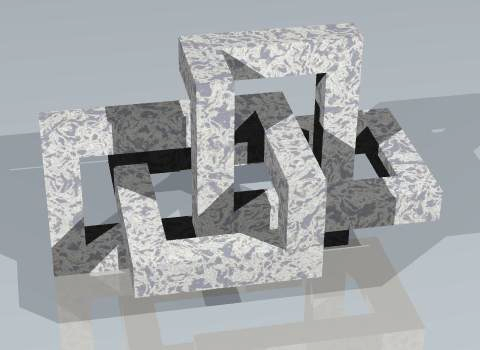
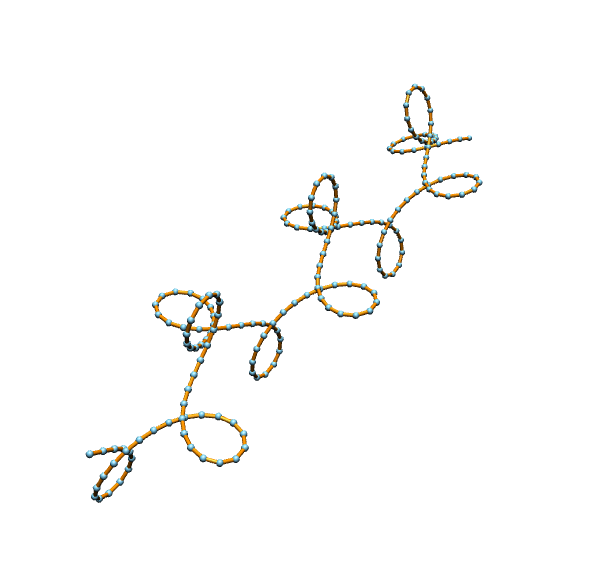
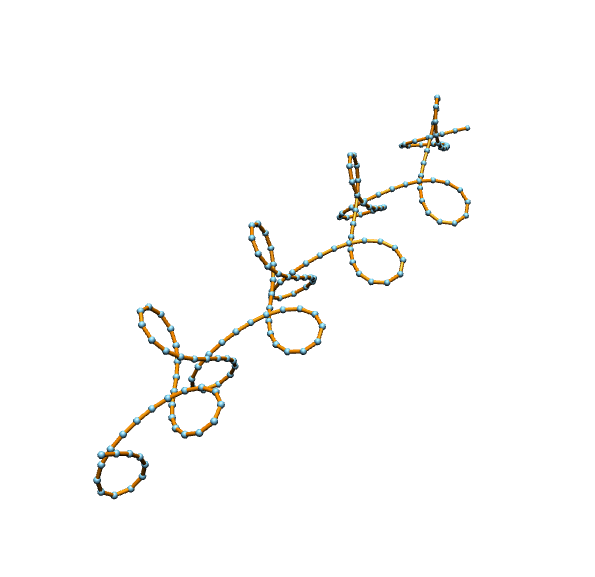
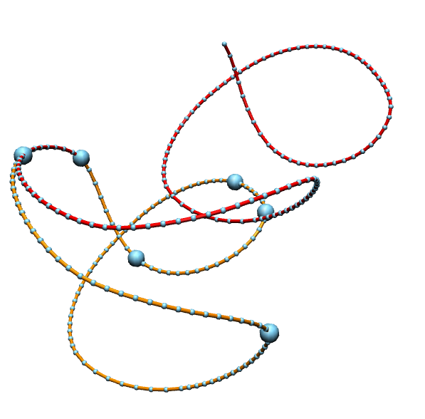
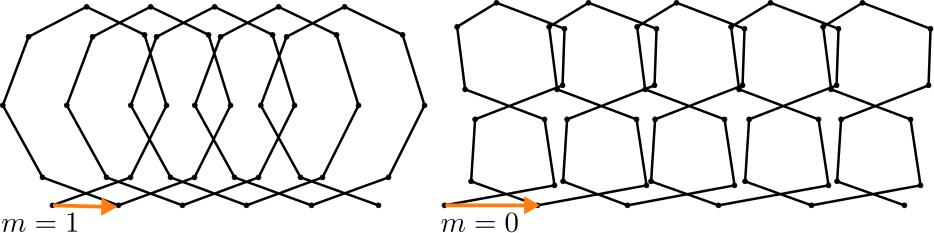
In order to produce nice pictures the appearance of the curves can be changed and the result can be exported as pdf. The following pictures show two examples.

 

If one really wants to understand what is going on, we need a bit more mathematical background.

Dual Curves

If we start with a smooth 1-parameter family of lines \(L\) in the plane, then there is a smooth curve \(\gamma\) such that \(\gamma\) is tangent to each curve in the family at some point – this curve \(\gamma\) is called the envelope of \(L\). The whole story directly translates to the discrete world. If you have a sequence of lines in the plane \(L\), then there corresponds a discrete curve \(\gamma\) to it. The construction of \(\gamma\) is elementary: two successive lines have an intersection. This gives a sequence of points, i.e. a discrete curve.

But wait, where do two parallel lines intersect? Right, they do not intersect in \(\mathbb{R}^2\), but in an infinitely far “ideal” point. If want to make this precise, we have to speak about the real projective plane. Here every pair of distinct lines intersects in exactly one point. We will give a short impression. For a serious treatment see the literature. There are lots of books on this subject. I recommend the lecture notes of Nigel Hitchin on projective geometry and quadrics, which are free available on his homepage http://people.maths.ox.ac.uk/hitchin/.

Real Projective Space. The \(n\)-dimensional real projective space consists of all (unoriented) lines through the origin of a \(n+1\)-dimensional real vector space \(V\). To make this more rigorous, introduce an equivalence relation \(\sim\) on \( V_0:= V\setminus\{0\}\) as follows\[ x\sim y:\Leftrightarrow x= \lambda y ,\quad 0\not=\lambda\in\mathbb{R}.\]

We denote the equivalence class of a vector \(x\) by \([x]\). The \(n\)-dimensional real projective space \(P(V)\) is then the quotient space with respect to the defined equivalence relation:\[ P(V)= V_0/_\sim.\]

If \(V\) is 2-dimensional we call \(P(V)\) a projective line. If \(V\) is 3-dimensional we call it a projective plane.

Curves in the Projective Plane. For now we are only interested in the projective plane \(\mathbb{RP}^2= P(\mathbb{R}^3)\). Each plane \(U\subset\mathbb{R}^3\) in \(\mathbb{R}^3\) can be identified with \(\mathbb{R}^2\). If \(U\) does not contain the origin, each point in \(U\) can be identified with a point in \(\mathbb{RP}^2\) by \(x \mapsto [x]\). The points in \(\mathbb{RP}^2\) which are not obtained this way are exactly the vectors that are parallel to \(U\). This is a 2-dimensional subspace of \(\mathbb{R}^3\) – the projectivization of which is a real projective line. Hence, we can consider the real projective plane as the union of \(\mathbb{R}^2\) with a real projective line \(\mathbb{RP}^1\) – the “ideal line”:\[ \mathbb{RP}^2= \mathbb{R}^2\cup \mathbb{RP}^1.\]

In this sense each plane curve \(\gamma=(\gamma_1,\gamma_2)\) lifts to a projective one. If we choose \(U= \{x\in\mathbb{R}^3\mid x_3=1\}\) then the map is simply given by \[ \gamma \mapsto \Gamma = [\gamma_1,\gamma_2,1]. \]

Opposite, if we have a projective curve \(\Gamma=[\Gamma_1,\Gamma_2,\Gamma_3]\) that does not pass the ideal line, i.e. \(\Gamma_3\not= 0\), then we can get corresponding curve in \(\mathbb{R}^2\) by normalizing the last component to \(1\):\[ \Gamma \mapsto \gamma= (\Gamma_1/\Gamma_3,\Gamma_2/\Gamma_3).\]

If \(\Gamma\) is a general projective curve, we call the part which does not intersect the ideal line the finite part of \(\Gamma\).

Curves of lines. What does this have to do with families of lines in \(\mathbb{R}^2\)? A line \(L\) in the real plane can given by an equation\[ L_{(a,b,c)}=\{(x,y)\in \mathbb{R}^2 \mid ax+by-c=0\}\quad a,b,c\in \mathbb{R}.\]

So we see that lines are essentially given by vectors in \(\mathbb{R}^3\). But the equation can be multiplied by an arbitrary non-zero scalar while the line does not change. Thus the line corresponds to a point in the projective plane.

How the line can be recovered from that point \([a,b,-c]\in\mathbb{RP}^2\)? Consider the linear form \[ \eta_{(a,b,c)} (x,y,z) = ax+by-cz. \]

The projectivization of its kernel is a projective line the finite part of which is exactly \(L_{(a,b,c)}\).

So we have seen that plane curves and smooth families of lines both can be regarded as curves in the projective plane.

Polarity. Let \(Q\) be an indefinite non-degenerate quadratic form on \(\mathbb{R}^3\). By Sylvester’s law of inertia every such form on \(\mathbb{R}^3\) arises from a standard form by a change of basis. We can assume without loss of generality that the form is represented by the matrix the following matrix: \[Q=\begin{pmatrix} 1&0&0\\ 0&1&0\\ 0&0&-1 \end{pmatrix}.\]

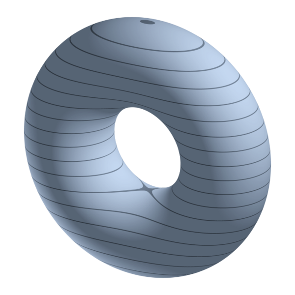
The quadric \(\mathbf Q \subset \mathbb{RP}^n\) is defined as the zero set of \(Q\), i.e.\[ \mathbf Q= \{[x]\in \mathbb{RP}^2 \mid Q(x,x)=0\}.\]

Note, that the zero set is also well defined in the projective setting. The intersection with the plane \(\{z=1\}\) is just a round circle. If one instead intersects it with other planes one gets the usual plane conic sections as shown in the picture below.

With \(Q\) we get an isomorphism from \(\mathbb{R}^3\) to \(\mathbb{R}^3\). It is given by the following map\[ (a,b,c)\mapsto (a,b,-c).\]

Under this map the point \((a,b,c)\) is identified with \(L_{(a,b,c)}\), called the polar of the point. The correspondence has also a nice geometric construction as shown in the next picture (taken from here).

Using this duality we get for each projective curve \(\gamma\) a dual projective curve \(\Gamma\).

The dual curve \(\Gamma\) of a curve \(\gamma\) in \(\mathbb{R}^2\) is defined as the envelope of the line field corresponding to the dual curve of the projective curve induced by \(\gamma\). Hopefully, this won’t lead to confusion.

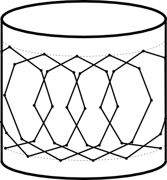
The curve does not have to stay in the finite part, but can also pass the ideal line as shown in the picture below.

The evolute of a curve

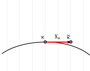
Smooth case. Let \(\gamma\) be a plane curve. The evolute of \(\gamma\) is defined as the envelope of the normal field of \(\gamma\). It can be shown that the evolute \(\hat\gamma\) is given by \[ \hat\gamma= \gamma+\tfrac{1}{\kappa}N,\] where \(N\) denotes the normal field and \(\kappa\) the curvature of \(\gamma\). If \(\gamma\) was arclength parametrized \(\kappa\) is given by\[ T^\prime= \kappa N. \]

The osculating circle of \(\gamma\) is the circle that touches \(\gamma\) of second order. Its center \(c_\kappa\) is called the center of curvature. Its radius \(R\) and \(\kappa\) are related by\[ R= \left|\tfrac{1}{\kappa}\right|. \] In other words: The evolute is the trace of the center of curvature.

Discrete case. While it is clear what the normal field is in the smooth case, there are different possible choices of normal directions in the discrete case. It is even not clear whether they sit at vertices or on the edges, but there are good possible choices.

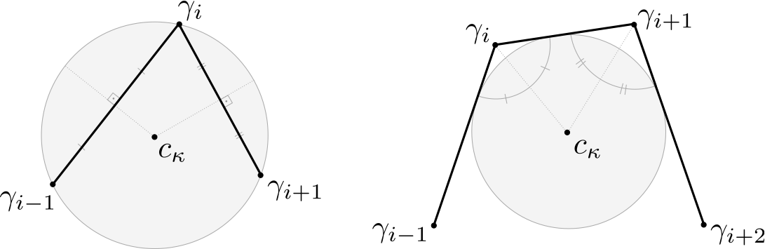
Possibility 1: Define the normal spaces at edges. Here the most obvious choice is to take the edge bisector (see here e.g.). The edge bisectors of two successive edges meat in the circumcenter of the triangle that is determined by the two involved edges.

Hence one possibility of a discrete evolute is to define it as the sequence of circumcenters of three successive vertices.

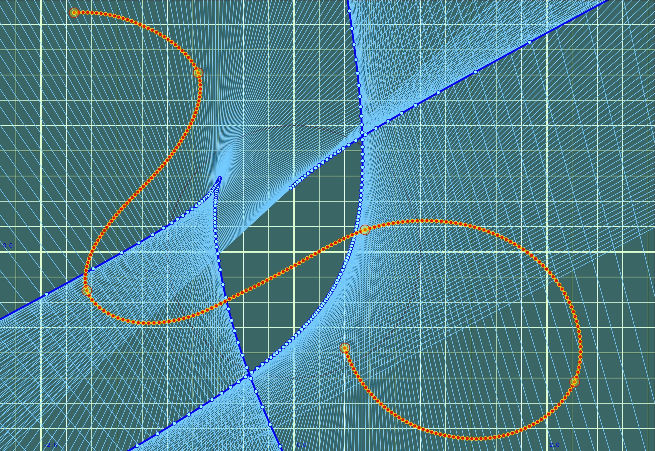
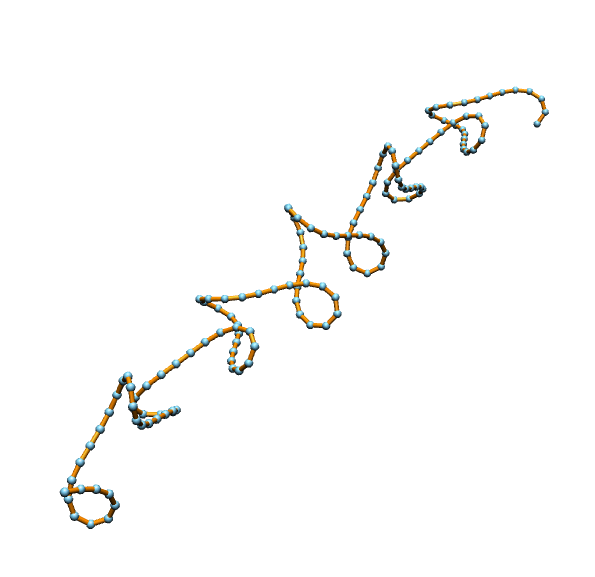
In fact, we can easily translate that into the projective curve setting, i.e. we can specify the normal field by a projective curve. Drawing the envelope yields nice results. Below you find two examples of evolutes defined using edge bisectors.

 

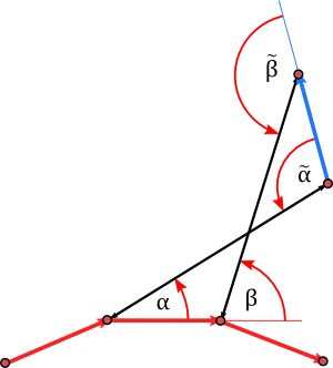
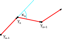
Possibility 2: Define the normal spaces at vertices. Here the angle bisectors that cross the discrete curve seem to be a good choice. The angle bisectors of two successive vertices meat in the center of a circle that touches the three edges that incident with the vertices – another osculating circle.

Homework: Implement both definitions of a discrete evolute, i.e. write a plugin that can switch between the two definitions. Use for it the DualPolygon2D class, which allows you to specify a projective curve, which interprets a dual projective curve as a curve of lines in the plane. The envelope is drawn automatically.