Let $\gamma_1,\ldots,\gamma_n\in \mathbb{R}^3$ be a regular discrete space curve. We are looking for another discrete space curve $\tilde{\gamma}$ that satisfies the first two conditions we had in the planar case: The distance between corresponding points $|\tilde{\gamma}_j-\gamma_j|$ is a constant $\ell$ and corresponding edges of $\gamma$ and $\tilde{\gamma}$ have the same length. Then (with a notation as in the previous post) we see that compared two the planar case we have a whole one-parameter family of possible choices for $S_{j+1}$: The vector $S_{j+1}$ can be the result of rotating $S_j$ around $\ell S_j + v_j T_j$ by any chosen angle.

One can imagine to start with a parallelogram with sides $v_j T_j$ and $\ell S_j$. The parallelogram is then folded around the diagonal whose direction is $\ell S_j-v_jT_j$.

Folding by 180 degrees corresponds to the Darboux-transformations we studied in the two-dimensional setting. It is given by the map

\[y\mapsto (\ell S_j-v_jT_j)y(\ell S_j-v_jT_j)^{-1}.\]

Any other folding angle (except for angle zero that would leave us with the parallelogram) can be realized as

\[y \mapsto qyq^{-1}\]

with $q$ of the form

\[q=r+\ell S_j-v_jT_j.\]

Here $r$ is an arbitrary real number. This leads to

\[S_{j+1}=(r+\ell S_j-v_jT_j)S_j(r+\ell S_j-v_jT_j)^{-1}\].

Definition: A discrete space curve $\tilde{\gamma}$ is called a Darboux transform of $\gamma$ with rod length $\ell$ and twist $r$ if

\[\gamma_j=\gamma_j+\ell S_j\]

and $S_1,\ldots, S_n$ satisfy the above equation.

Let us omit the subscript $j$ and use a subscript “+” instead of $j+1$. Combining then in the above formula the $S$ in the middle with the left bracket we see that the map $S\mapsto S_+$ is fractional linear:

\[S_+=((r -v T) S-\ell)((r -vT)+\ell S)^{-1}.\]

To investigate this map further we write $S$ as the stereographic projection with center $-T$ of some point $Z\in \mathbb{R}^3$ orthogonal to $T$:

\begin{align*} S &=(1-ZT)T(1-ZT)^{-1} \\\\ &=(T+Z)(1-ZT)^{-1} \\\\ &= T(1-ZT)(1+ZT)^{-1}.\end{align*}

The first line shows that $S\in S^2$ for $Z\perp T$. The second line shows that $Z\mapsto S$ is fractional linear. The last line shows that $S=Z$ in case $|Z|=1$. Let us plug this into the last formula for $S_+$:

\begin{align*}S_+&= ((r-vT)(T+Z)-\ell (1-ZT)((r-vT)(1-ZT)+\ell(T+Z))^{-1} \\\\ &=(((v-\ell)+rT)+(r-(v+\ell)T)Z)((r+(\ell-v)T)+((\ell+v)+rT)Z)^{-1} \\\\ &= \left(T+Z\frac{(\ell+v)-rT}{(\ell-v)-rT}\right)\left(1+TZ\frac{(\ell+v)-rT}{(\ell-v)-rT}\right)^{-1}.\end{align*}

Here the fractional notation is justified because the quaternions involved all commute. Thus in terms of the sterographic coordinate $Z$ the transition from $S$ to $S_+$ is just multiplication

\[Z+=MZ=Z\overline{M}\]

by a quaternion

\[M = \frac{(\ell+v)+rT}{(\ell-v)+rT}.\]

In the case $r=0$ this is in perfect accordance with the results of an earlier post.

Let us first look at the smooth case. Let \(\gamma\colon I\to \mathbb{R}^3\) be an arc length parameterized smooth curve with tangent vector \(T:=\gamma^\prime\).

An adapted frame is then a smooth map \(\sigma\colon I\to SO(3)\) such that \(\sigma e_1 = T\). We denote the second and the third column of \(\sigma\) by \(N\) and \(B\)\[\sigma= (T,N,B).\]The fields \(N\) and \(B\) are normal vector fields. Clearly \(B=T \times N\).

Let us take the derivative of \(\sigma\). Since the vectors \(T,N,B\) are normalized we find that\[\sigma^\prime=\sigma \mathcal{U},\]where\[\mathcal{U}=\begin{pmatrix}0 & \kappa_1 & \kappa_2 \\ -\kappa_1 & 0 & -\tau \\ -\kappa_2 & \tau & 0 \end{pmatrix}.\]

If \(N\) is parallel along \(\gamma\), i.e. the derivative has only a tangential component \(N^\prime= \kappa_1 T\), then so is \(B\), and \(\tau\) vanishes:\[\mathcal{U}=\begin{pmatrix}0 & \kappa_1 & \kappa_2 \\ -\kappa_1 & 0 & 0 \\ -\kappa_2 & 0 & 0 \end{pmatrix}.\]Such a frame is called a parallel frame. We have seen in the lecture that parallel frames always exist.

If \(\sigma=(T,N,B)\) is a parallel frame and \(\alpha\in\mathbb{R}\), then we define a new frame \(\sigma_\alpha= (T,N_\alpha,B_\alpha)\) with \[N_\alpha = \cos\alpha\, N+ \sin\alpha\, B,\quad B_\alpha=-\sin\alpha\, N+ \cos\alpha\, B.\]This frame is parallel again.

The point now is that, up to Euclidean motion, \(\gamma\) is determined by \(\mathcal{U}\). We can just solve for \(\sigma\) and obtain \(T\) as its first column. The curve is then reconstructed by integrating \(T\).

The term spinning refers then to the following procedure. We start with a curve \(\gamma\) and a parallel frame \(\sigma\). This gives us \(\mathcal{U}\) with \(\kappa_1\) and \(\kappa_2\). Now we define \(\mathcal{U}_\lambda\) for \(\lambda\in\mathbb{R}\) as follows\[\mathcal{U}_\lambda=\begin{pmatrix}0 & \kappa_1 & \kappa_2 \\ -\kappa_1 & 0 & -\lambda \\ -\kappa_2 & \lambda & 0 \end{pmatrix}.\]This determines a new curve \(\gamma_\lambda\). This family of curves is called the associated family.

Our plan is to spin discrete space curves. So let \(\gamma=(\gamma_0,\dots,\gamma_n)\) be a discrete space curve. Thinking of linear interpolation one finds the best place to locate an adapted frame is on the edges. Here it is clear what the tangent \(T_i\) shall be\[\gamma_i^\prime:=\gamma_{i+1}-\gamma_i= \ell_i T_i.\]

Since the tangent on each edge is constant, we can put just a constant frame on each edge, i.e. for each edge we get \(\sigma_i\) such that \(\sigma_i e_1= T_i\). Only at vertices the frame field has to jump.

We define a discrete adapted frame as a collection of \(SO(3)\)-matrices \(\sigma_i\) such that \(\sigma_i e_1= T_i\).

The jumps over the vertices are again given by \(SO(3)\)-matrices \(\mathcal{U}_i\), which we will call transport matrices. Quiet analogue to the smooth we have\[\sigma_i= \sigma_{i-1} \mathcal{U}_i.\]

As in the smooth world the transport matrices determine the adapted frame. If a initial value \(\sigma_0\) is given then \(\sigma_i\) is given by\[\sigma_i=\sigma_0\mathcal{U}_1 \cdots\mathcal{U}_i.\]

The corresponding curve is then reconstructed by integration of \(T= \sigma e_1\). So we get for \(\gamma_0\in \mathbb{R}^3\) and \(\sigma_0\):\[ \gamma_{k+1} = \gamma_0 + \sigma_0 \bigl(\sum_{i=0}^k \ell_i\mathcal{U}_1 \cdots\mathcal{U}_i\bigr)e_1.\]

Again we find special transport matrices, namely these which change the frame as minimal as possible, i.e. if \(T_{i-1}\) and \(T_i\) are parallel then \(\mathcal{U}_i=Id\) and else \(\mathcal{U}_i\) rotates \(\sigma_{i-1}\) around \(T_{i-1}\times T_i\). These transport matrices we will denote by parallel transport. They come directly with the geometry of the curve.

A frame with such transport matrices is called a discrete parallel frame. Each discrete curve admits a parallel frame.

Now let \(\gamma\) be a discrete space curve with a parallel frame \(\sigma=(T,N,B)\). Then this defines complex numbers \(q\) at the vertices in the following way: Consider the vertex \(\gamma_{i+1}\). The plane \(\mathcal{N}_{i}\) spanned by the vectors \(N_{i},B_{i}\) can be considered as complex line with rotation given by 90-degree-rotation around \(T_{i}\) which we will denote by \(J\), i.e. \(JX=T_i\times X\). The next tangent vector \(T_{i+1}\) lies on the unit sphere with the point \(-T_{i}\) removed.

If we perform stereographic projection with respect to the north pole \(-T_{i}\), then the tangent vector \(T_{i+1}\) is mapped to \(\mathcal{N}_i\) and hence defines a complex number \[q_{i+1}=\kappa_1\, N_i + \kappa_2 B_i=(\kappa_1 + \kappa_2 J) N_i.\] This can be interpreted as discrete complex curvature.

If the tangents are linearly dependent then \(q=0\). If they are not they span a plane. We slice the sphere by this plane and find that the magnitude of \(q\) is given by\[|q|= \tan(\tfrac{\alpha}{2}),\]where \(\alpha\) is the angle between \(T_i\) and \(T_{i+1}\).

In general frames can have torsion. While the curvature is located at the vertices, we define the torsion on the edges. Let \(\sigma\) be an arbitrary frame. Imagine the frames located at the start of the edges. We want to know how much it rotates around the edge from the beginning to the end. To get the rotation angle we use the parallel transport to pull the frame on the next edge back to the end of the current. I.e. we have \(\sigma_i\) and \(\sigma_{i+1}\mathcal{U}_{i+1}^{-1}\), both adapted to the i-th edge. They differ by a rotation around \(T_i\). If \(\alpha\) is the angle of the rotation, then the torsion \(\tau_i\) is given by \[\alpha= \tau_i \ell_i.\]

To go further, we change to quaternionic frames in which the transports takes a much simpler form. Therefore we identify \(\mathbb{R}^3\) with the imaginary quaternions, i.e.\[x_1e_1+x_2e_2+x_3e_3 \longleftrightarrow x_1\mathbf{i}+ x_2\mathbf{j}+x_3\mathbf{k}.\]With this identification a rotation around an axis given by a vector \(X\) with \(|X|=1\) by an angle \(\alpha\) takes the form\[P\mapsto X_\alpha PX_\alpha^{-1},\]where \[X_\alpha=\cos(\alpha/2)\mathbf{1} +\sin(\alpha/2)X.\]

So we can encode the frame equations by quaternions by considering \(\phi_i\) such that\[T_i = \phi_i\, \mathbf{i}\,\phi_i^{-1},\quad N_i = \phi_i\, \mathbf{j}\,\phi_i^{-1},\quad B_i = \phi_i\, \mathbf{k}\,\phi_i^{-1}.\]That is \(\phi\) rotates the standard basis to the basis given by the frame \(\sigma_i\). By the equations above \(\phi_i\) is determined up to a non-zero scale factor. As before the frames \(\phi_i\) are related by transports, i.e.\[\phi_{i}=\phi_{i-1}\mathcal{V}_i.\]

The reconstruction formula for the corresponding curve takes a quite similar form\[\gamma_{k+1}= \gamma_0 + \phi_0\bigl( \sum_{i=0}^{k}\ell_i (\mathcal{V}_1\cdots \mathcal{V}_i )\,\mathbf{i}\, (\mathcal{V}_1\cdots \mathcal{V}_i)^{-1}\bigr)\phi_0^{-1}.\]

Once we know the \(q\) the parallel transport takes an amazingly simple for in the quaternionic setting. It is given by \[\mathcal{V}_i = \mathbf{1}+ \mathbf{i}q\mathbf{j}= \mathbf{1}+ q\mathbf{k}= \mathbf{1} -\operatorname{Im}(q)\mathbf{j}+\operatorname{Re}(q)\mathbf{k}.\]

This is due to the fact that \(-\operatorname{Im}(q)\mathbf{j}+\operatorname{Re}(q)\mathbf{k}\) are the coordinates (wrt. \(\phi_{i-1}\)) of the rotation axis prescribed by parallel transport and \(|q|=\tan(\alpha/2)\), where \(\alpha\) is the rotation angle.

The rotation around the tangent takes the simple form \(\mathcal{T}_i^\alpha=\cos(\alpha\ell_i)\mathbf{1}+\sin(\alpha\ell_i)\mathbf{i}\). Hence we can spin the curve in the following way:

1. Take a parallel frame and calculate the corresponding \(q\)’s.
2. Define for \(\lambda\in \mathbb{R}\) a new parallel transport by \(\mathcal{V}^\lambda_i=\mathcal{T}^\lambda_{i-1}\mathcal{V}_i\).
3. Reconstruct the curve corresponding the \(\mathcal{V}^\alpha_i\).

Homework (due date 27 June): Your task is to implement the spinning procedure, i.e. write a plugin the constructs for a given \(\lambda\in\mathbb{R}\) the curve corresponding to the transports \(\mathcal{V}^\lambda_i\) as define above and adds it to the scene. The initial values should be chosen suitably.

As in the last post let $\gamma$ be a discrete curve in the $\mathbb{C}$ and $\tilde{\gamma}= \gamma+ \ell S$ be a Darboux transformation. Denote by $\alpha_j$ and $\beta_j$ the angles from the edges $T_J$ of $\gamma$ to the rod directions $S_j$ and $S_{j+1} respectively. Then

\begin{align*}S_j &= e^{i \alpha_j} T_j \\\\ S_{j+1}&= e^{i \beta_j} T_j.\end{align*}

We know that $S$ satisfies

\[ S_{j+1}=\frac{\ell S_j- v_j T_j}{\ell-v_j \bar{T}_j S_j}.\]

This yields

\[ e^{i\beta_j}=\frac{\ell e^{i\alpha_j}- v_j}{\ell-v_j e^{i\alpha_j}}.\]

Using the formula

\[e^{i\alpha}=\frac{1+it}{1-it}\]

where

\[t:=\tan \frac{\alpha}{2}\]

we then have

\begin{align*} e^{i\beta_j}&=\left(\ell \frac{1+it_j}{1-it_j}- v_j \right) \left(\ell-v_j \frac{1+it_j}{1-it_j} \right)^{-1} \\\\ &=\left(\frac{(\ell -v_j)+(\ell +v_j)it_j}{1-it_j}\right) \left( \frac{(\ell-v_j )-(\ell+v_j )it_j}{1-it_j} \right)^{-1} \\\\ &= \frac{1+i \mu_j t_j}{1-i \mu_j t_j} \,.\end{align*}

where

\[ \mu_j= \frac{\ell+v_j}{\ell-v_j}.\]

From this we conclude

\[\tan \frac{\beta_j}{2}=\mu_j \tan \frac{\alpha_j}{2}.\]

With the notation

\begin{align*}t_j&:=\tan \frac{\alpha_j}{2}\\\\ \tau_j&:=\tan \frac{\kappa_j}{2}\end{align*}

we obtain

\begin{align*}\tau_j&=\tan \frac{\beta_{j-1}-\alpha_j}{2}\\\\ &= \frac{\mu_{j-1} t_{j-1}-t_j}{1+\mu_{j-1} t_{j-1} t_j}.\end{align*}

The corresponding quantities for the Darboux transform $\tilde{\gamma}$ are

\begin{align*}\tilde{\alpha}_j &=\pi-\beta_j \\\\ \tilde{\beta}_j &= \pi- \alpha_j \\\\ \tilde{\tau}_j&=\tan \frac{\beta_j-\alpha_{j-1}}{2}\\\\ &= \frac{\mu_j t_j-t_{j-1}}{1+\mu_j t_j t_{j-1}}.\end{align*}

Note that we arrive at $\tilde{\tau}_j$ starting from $\tau_j$ if we interchange the roles of $t_{j-1}$ and $t_j$ and replace $\mu_{j-1}$ by $\mu_j$. If we apply this rule to

\begin{align*}1+\tau_j^2 &= \frac{(1+2\mu_{j-1} t_{j-1} t_j +\mu_{j-1}^2 t_{j-1}^2 t_j^2) + (t_j^2 -2 \mu_{j-1} t_{j-1} t_j +\mu_{j-1}^2 t_{j-1}^2)}{(1+\mu_{j-1} t_{j-1} t_j)^2} \\\\ &= \frac{(1+t_j^2)(1+\mu_{j-1}^2 t_{j-1}^2)}{(1+\mu_{j-1} t_{j-1} t_j)^2} \end{align*}

we obtain

\[1+\tilde{\tau}_j^2=\frac{(1+t_{j-1}^2)(1+\mu_j^2 t_j^2)}{(1+\mu_j t_j t_{j-1})^2}\]

Now the following is easy to prove:

Theorem: If $\gamma$ is a closed polygon in $\mathbb{R}^2$ with equal edge lengths and $\tilde{\gamma}$ is a closed Darboux transform of $\gamma$ then

\[\prod_{j=1}^n (1+\tau^2) = \prod_{j=1}^n (1+\tilde{\tau}^2).\]

We can interpret this as follows: The bending energy

\[\sum_{j=1}^n \log (1+\tau_j^2)=-\sum_{j=1}^n \log (1+\cos \kappa_j)\]

is the same for $\gamma$ and $\tilde{\gamma}$.

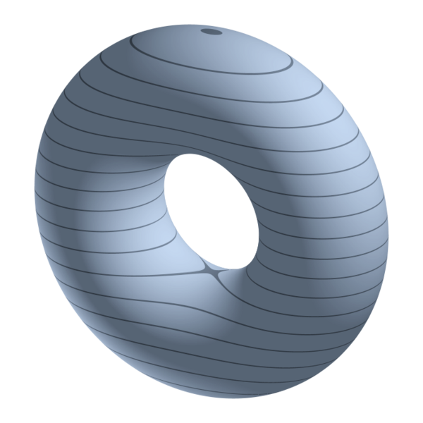
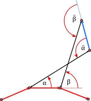
As we saw in the  lecture, we can parametrize the moduli space of discrete closed plane curves by angles and edge lengths, which encode how the tangent is moving along the curve. More explicit: up to rigid motion each discrete curve with \(n\) vertices and tangent winding number \(m\) is represented by a point in a submanifold \(\mathcal{M}_0\) of \((-\pi,\pi)^{n}\times (0,\infty)^{n}\), which is given by the zero set of the map \[ F:(-\pi,\pi)^{n}\times (0,\infty)^{n} \to \mathbb{R}^3 = \mathbb{R}\times \mathbb{C}\\\\ F(\ell,\kappa)=\left(\begin{array}{c} \kappa_1+\ldots +\kappa_n -2 \pi m \\  \ell_1 e^{i\alpha_1}+\ldots +\ell_{n}\, e^{i\alpha_{n}}\end{array}\right),\] where \[\alpha_j= \kappa_1+\ldots+\kappa_j.\]

In general, each function defined on \(\mathcal{M}\) splits the space into components. E.g. think  of a height function of an embedded surface.

If the map is ‘nice’ enough, i.e. in our case smooth and of constant rank, then the level sets are submanifold. Moreover \(\mathcal{M}_0\) is the intersection of the submanifolds \(\mathcal{M}_1\) and \(\mathcal{M}_2\), which are given as zeros sets of the functions\[F_1(\ell,\kappa)=\kappa_1+\ldots +\kappa_n -2 \pi m, \quad F_2(\ell,\kappa)=\ell_1 e^{i\alpha_1}+\ldots +\ell_{n}\, e^{i\alpha_{n}}.\]

Now, we have given \(\mathcal{M}_0\) which parameterizes discrete closed plane curves. But what does the ambient space correspond to?

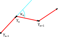
It is important to note that a closed curve is in fact rather a periodic sequence of points than just \(n\) points. With this in mind, let us assign to each point in \((-\pi,\pi)^{n}\times (0,\infty)^{n}\) periodic sequences, denoted again by \(\kappa\) and \(\ell\), to which corresponds a discrete curve \(\gamma \colon \mathbb{Z}\to \mathbb{C}\). The curve \(\gamma\) is obtain by ‘integration’, i.e. e.g. for positive \(k\) we have\[\gamma_{k+1}=\sum_{j=1}^k \ell_j e^{i\alpha_j}.\]

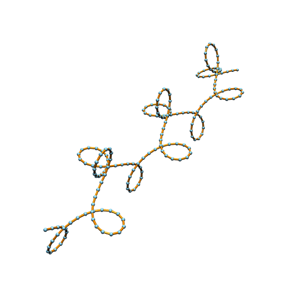
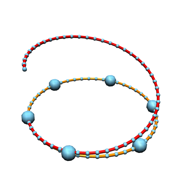
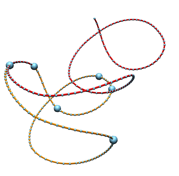
Now we can directly look at the effect of dropping conditions: Let us start outgoing from the case that \(\kappa,\ell\) lies on \(\mathcal{M}_0\), i.e. we have a discrete closed plane curve as shown below.

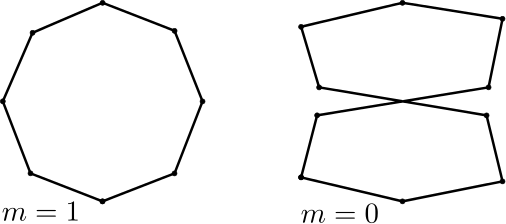
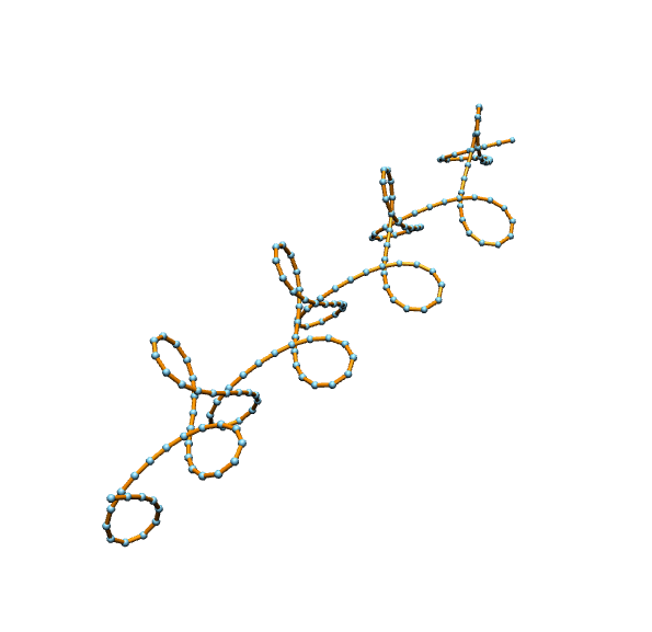
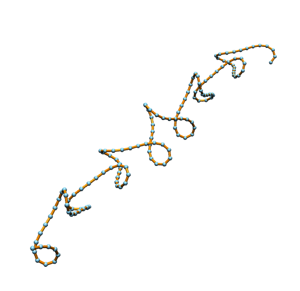
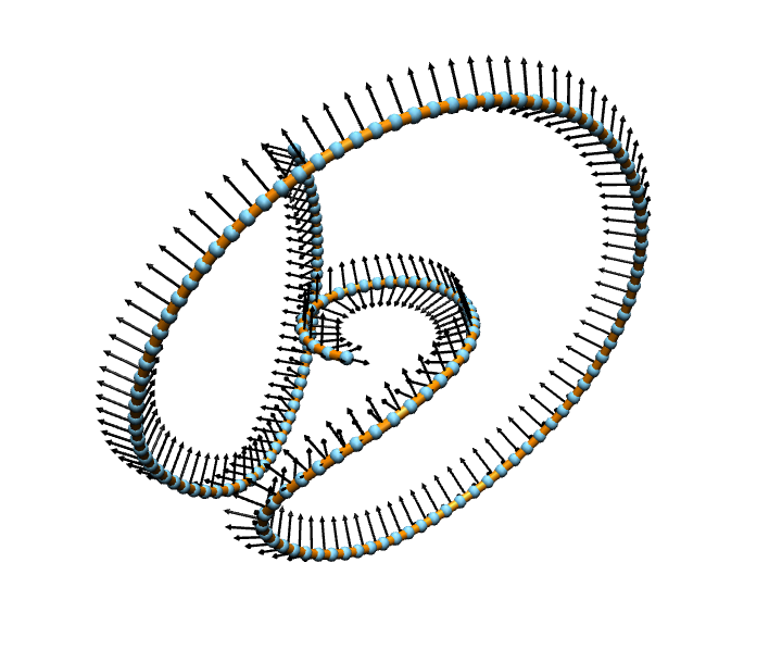
If we drop the second condition we just stay on \(\mathcal{M}_1\), i.e. the curves do not have to close up but the tangent winding number is still restricted to \(2\pi m\), such curves are know as curves with translational period. Examples are shown below.

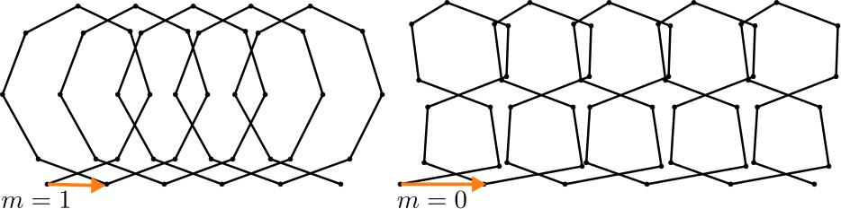
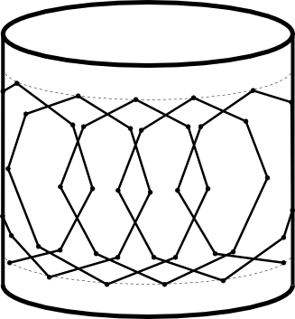
These curves can also regarded as closed curves on a cylider.

Our task is now to navigate on the submanifold \(\mathcal{M_0}\), i.e. given a vector field \(X\) on \(\mathcal{M_0}\) and a point \(p \in\mathcal{M_0}\), then move along the integral curve of \(X\) starting at \(p\).

In our setup we are surrounded by a Euclidean space that means that tangent vector fields are just maps into \(\mathbb{R}^{2n}\). First, let us ignore all conditions for a moment. Then we can just use the Euler method to follow the vector field, i.e. we just go a bit in the direction of the vector field: If at time \(t\) we are at the position \(p(t)\), then \[ p(t+\varepsilon)= p(t)+\varepsilon X(p(t)),\] is the position at time \(t+\varepsilon\). Since this shall correspond to a discrete curve that was obtained by regular homotopy we have to ensure that we don’t leave the open subset \((-\pi,\pi)^{n}\times (0,\infty)^{n}\). But that’s easy.

It is also easy to stay in \(\mathcal{M}_1\) as it consists of open subsets of affine vector spaces, i.e. all one has to do is to project the given vector field \(X\) to the tangent space of \(\mathcal{M}_1\). If \(X^\top\) denotes the projection, the corresponding line \(p+\operatorname{span}\{X^\top(p)\}\) is then already contained in the affine vector space. Again all we have to ensure is that the point does not leave an open set.

The situation changes if we start at a closed curve \(p(t)\) and want to stay closed. First, the vector field then has to be tangential to \(\mathcal{M}_0\), i.e. we have to eliminate the normal components. Second, even if the field is tangential, we will leave \(\mathcal{M_0}\) Immediately if we move along a line. Our strategy will be to fix this by projecting back to \(\mathcal{M_0}\) after each Euler step.

Let us focus on the situation that all lengths shall stay fixed during the flow as it was presented in the lecture, i.e. all components of the vector field that correspond to lengths are just zero:\[X(p)=(X_1(p),\dots,X_{n}(p),0,\dots,0).\]

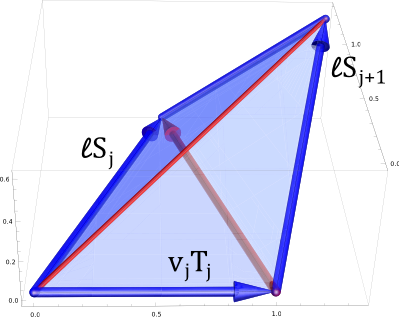
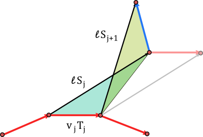
The normal space to \(\mathcal{M}_0\) at a point \(p=(\kappa_1,…,\kappa_{n},\ell_0,…,\ell_{n}) \in \mathcal{M}_0\) was spanned by \[V_0=(1,\dots,1,0,\dots,0)\] and the vertex coordinates of a curve \(\gamma\) corresponding to the point \(p\) \[ V_1=(x_1,\dots,x_j,0,\dots,0),\\ V_2=(y_1,\dots,y_j,0,\dots,0),\] where the \(x_j\) and \(y_j\) denotes the real and imaginary part of \(\gamma_j\) resp., i.e. \(\gamma_j=x_j+iy_j\).

We apply the Gram-Schmidt process starting with \(V_0\) and obtain an orthonormal basis \(N_0,N_1,N_2\) of the normal space of \(\mathcal{M}_0\). The projection of \(X\) on its tangential part \(X^T\) then takes the simple form\[X^\top=X-\sum_{j=0}^2\langle X,N_j\rangle N_j.\]

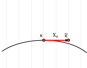
We perform the Euler step with respect to the field \(X^\top\) and obtain a new point \(\tilde p=(\tilde\kappa,\ell)\) which a priori not yields a closed curve. Now we have to get back to \(\mathcal{M}_0\), i.e. we have to change the \(\tilde\kappa\) slightly so that \(F(\tilde\kappa,\ell)=0\). Hence we have to search for a zero of a non-linear function in an \(n\)-dimensional space, which in general is slow and the speed moreover depends on the number of vertices.

We reduce this problem, as proposed, to a \(2\)-dimensional one by projecting \(\tilde p\) back along the normal space at the previous point \(p\):\[f(\lambda_1,\lambda_2)=F(\tilde\kappa+\lambda_1N_1+\lambda_2 N_2,\ell)=0.\]

This we solve by applying the Newton method and obtain a new closed curve.

Homework (due date 6 June): Your task is to implement the gradient flow of the bending energy on closed curves. In the repository you find under de.jtem.discreteCurves.tutorial a class called GradientFlowPlugin which provides a basic environment to start with. It shows the gradient flow of the bending energy\[E(\kappa,\ell)= \tfrac{1}{2}\sum_{j=1}^{n} \kappa_j^2.\] without any constraints, i.e. closed curves immediately open up and are deformed into straight lines.

Copy the GradientFlowPlugin into your project.

Your task is now to modify the flow so that closed curves stay closed, i.e. you have the following things to do:

1. Project the gradient of the bending energy to the tangent space of \(\mathcal{M}_0\) to obtain a vector field \(X\) which is tangential.
2. Implement the projection back to \(\mathcal{M}_0\) after the Euler step.

The Euler step just stays as it is. For the second item you can use the Newton method that is implemented in the jtem project numericalMethods (explicitly in de.jtem.numericalMethods.calculus.rootFinding).

Hint: Even if it is not an example for the usage of the Newton-class it may be helpful to look into ExampleNewtonRaphson, which you find at the same place.

In this post we will work with a fixed sequence of lengths  $\ell_1,\dots,\ell_n>0$. This means we imagine polygons as composed of rigid edges connected by flexible joints at the vertices. Denote by $\mathcal{M}_m$ the space of curvature functions $\kappa=(\kappa_1,\ldots,\kappa_n)$ that correspond to closed regular polygons with $n$ vertices and tangent winding number $m$.  We can conveniently describe $\mathcal{M}_m$ as the zero set of the function

\begin{align*}\qquad F:(-\pi,\pi)^n &\to \mathbb{R}^3 = \mathbb{R}\times \mathbb{C}\\\\ F(\kappa_1,\ldots,\kappa_n)&=\left(\begin{array}{c} \kappa_1+\ldots +\kappa_n -2 \pi n \\  \ell_0 e^{i\alpha_0}+\ldots +\ell_{n-1}\, e^{i\alpha_{n-1}}\end{array}\right).\end{align*}

By the above calculation the derivative of $F$ is given as

\[F'(\kappa_1,\ldots,\kappa_n)\left(\begin{array}{c}\dot{\kappa}_1\\ \vdots \\ \dot{\kappa}_n\end{array}\right)=\left(\begin{array}{c} \dot{\kappa}_1+\ldots +\dot{\kappa}_n \\ \dot{\kappa}_1 \gamma_1+\ldots + \dot{\kappa}_n \gamma_n \end{array}\right).\]

Theorem: The rank of $F’$ is three at all points of $\mathcal{M}_m$. Therefore, by the implicit function theorem, $\mathcal{M}_m$ is a smooth manifold.

Proof: At a point $(\kappa_1,\ldots,\kappa_n)$ where the columns of $dF(\kappa_1,\ldots,\kappa_n)$ were linearly dependent we would have $a,b,c\in \mathbb{R}$ such that

\[a \mbox{Re}(\gamma_j)+b \mbox{Im}(\gamma_j)+c=0\]

for all $j$. But this means that the whole polygon lies on a straight line, which is impossible for a regular polygon.

$\square$

Suppose we have a vector field tangent to $\mathcal{M}_m$ that we want to follow numerically. This means that for any $\kappa=(\kappa_1,\ldots,\kappa_n)\in \mathcal{M}_m$  we are given a certain tangent vector

\[X_\kappa \in T_\kappa \mathcal{M}_m=\mbox{ker}F'(\kappa).\]

We want to find curves $t\mapsto \eta(t)\in \mathcal{M}_m$ that satisfy for all $t$

\[\dot{\eta}(t)=X_\eta(t).\]

If we already have constructed $\kappa=\eta(t)$ we might attempt to find $\eta(t+\epsilon)$ as

\[\tilde{\kappa}=\kappa+\epsilon \dot{\kappa}\]

where $\dot{\kappa}=X_{\kappa(t)}$. Since $\dot{\kappa}$ lies in the kernel of $F'(\kappa)$ the condition

\[\tilde{\kappa}_1+\ldots+\tilde{\kappa}_n=2\pi m\]

will be satisfied. The second condition

\[\ell_0 e^{i\tilde{\alpha}_0}+\ldots +\ell_{n-1} \,e^{i\tilde{\alpha}_{n-1}}\]

however is non-linear and so we cannot be sure that $\tilde{\kappa}$ corresponds to a closed regular polygon. We first have to project $\tilde{\kappa}$ back to $\mathcal{M}_m$.

To this end we add to $\tilde{\kappa}$ an element of $(T_\kappa\mathcal{M}_m)^\perp$, the normal space to $\mathcal{M}_m$ at the point $\kappa$. This space is spanned by

\begin{align*}N_0&=(1,\ldots,1)\\\\ N_1&=(x_1,\ldots,x_n) \\\\ N_2 &=(y_1,\ldots,y_n)\end{align*}

Here $\gamma_j=x_j+iy_j$ and we assume that a translation has been applied to $\gamma$ in order to achieve

\[\gamma_1+\ldots,+\gamma_n=0.\]

Since the condition $\tilde{\kappa}_1+\ldots+\tilde{\kappa}_n=2\pi m$ already has been dealt with there is no need to work with $N_1$. We therefore are looking for $\lambda_1,\lambda_2 \in \mathbb{R}$ such that

\[f(\lambda_1,\lambda_2)=(0,0).\]

Here

\[f(\lambda_1,\lambda_2)=G(\kappa+\lambda_1 N_1 + \lambda_2 N_2)\]

where

\[G(\hat{\kappa}):=\ell_1e^{i\hat{\alpha}_1}+\ldots+\ell_{n-1}e^{i\hat{\alpha}_{n-1}}\,.\]

Thus we are left with the problem of finding a zero of $f$. From the calculation at the beginning of the post we know the derivative of $f$, so a Newton method seems the right thing to implement.

The moduli space (meaning congruent polygons are considered as equal) of open regular polygons $\gamma_0,\ldots,\gamma_n$ in the plane can be parametrized by parameters

\[(\ell_0,\ldots,\ell_{n-1},\kappa_1,\ldots,\kappa_{n-1})\in (0,\infty)^{n-1} \times (-\pi,\pi)^{n-2}.\]

If we we want to construct an actual polygon from such data we first define $\alpha_0,\ldots,\alpha_{n-1}$ as

\[\alpha_j=\kappa_1+\ldots+\kappa_j.\]

From these we define normalized edge vectors $T_j=e^{i\alpha_j}$ and finally the polygon itself: For $j=0,\ldots,n$ we set

\[\gamma_j=\ell_0 T_0+\ldots+\ell_{j-1} T_{j-1}.\]

The direction of the edge joining $\gamma_j$ to $\gamma_{j+1}$ is given by $T_j=e^{i\alpha_j}$ with . Then the position $\gamma_n$ of the last vertex (equal to $\gamma_0$ for a closed polygon) is given a

\[\gamma_n=\ell_0 e^{i\alpha_0}+\ldots +\ell_{n-1} e^{i\alpha_{n-1}}.\]

Theorem (Schläfli Formula): From given parameters

\[(\ell_0,\dots,\ell_{n-1},\kappa_1,\ldots,\kappa_{n-1})\in (0,\infty)^{n-1} \times (-\pi,\pi)^{n-2}\]

construct a polygon $\gamma_0,\ldots,\gamma_n$ as described above. Consider a variation $(\dot{\ell}_0,\dots,\dot{\ell}_{n-1},\dot{\kappa}_1,\ldots,\dot{\kappa}_{n-1})$ of these parameters and define

\[\dot{\kappa}_n:=-(\dot{\kappa}_1+\ldots+\kappa_{n-1}).\]

Then the corresponding variation of $\gamma_n$ will be given by

\[\dot{\gamma}_n=\sum_{j=0}^{n-1} \, \dot{\ell}_j T_j-i \sum_{j=1}^{n}  \dot{\kappa}_j \gamma_j.\]

Proof: For $j=0,\ldots,n$ define $\dot{\alpha}_j:=\sum_{k=1}^j \,\dot{\kappa}_k$.

Then $\dot{\alpha}_0=\dot{\alpha}_n=0$ and

\begin{align*}\dot{\gamma}_n &=\sum_{j=0}^{n-1} \, (\dot{\ell}_j +i\ell_j \dot{\alpha}_j) e^{i\alpha_j}\\\\ &= \sum_{j=0}^{n-1} \, \dot{\ell}_j T_j +i \sum_{j=1}^{n-1}  \dot{\alpha}_j (\gamma_{j+1}-\gamma_j) \\\\ &=  \sum_{j=0}^{n-1} \, \dot{\ell}_j T_j+i \dot{\alpha}_{n-1}\gamma_n -\dot{\alpha}_1 \gamma_1-i \sum_{j=2}^{n-1}  (\dot{\alpha}_j-\dot{\alpha}_{j-1}) \gamma_j\\\\ &=\sum_{j=0}^{n-1} \, \dot{\ell}_j T_j-i (\dot{\alpha}_n-\dot{\alpha}_{n-1})\gamma_n -i(\dot{\alpha}_1-\dot{\alpha_0}) \gamma_1-i \sum_{j=2}^{n-1}  \dot{\kappa}_j \gamma_j\\\\  &=\sum_{j=0}^{n-1} \, \dot{\ell}_j T_j-i \sum_{j=1}^{n}  \dot{\kappa}_j \gamma_j.\end{align*}

$\square$

Let $(\gamma_0,\ldots,\gamma_n)$ be a regular polygon in the plane $\mathbb{R}^2$. Then there are unique real numbers $\ell_0, \ldots ,\ell_{n-1}>0$ and unit vectors $T_0,\ldots,T_{n-1}\in S^1$ such that the edge vectors of $\gamma$ have the form

\[\gamma_{j+1}-\gamma_j=\ell_j T_j.\]

Furthermore, it never happens that $T_{j+1}=-T_j$ and therefore there are unique real numbers $\kappa_1,\ldots,\kappa_{n-1}$ such that

\begin{align*}-\pi &< \kappa_j < \pi \\\\ T_j &= e^{i\kappa_j}\,T_{j-1}.\end{align*}

It is easy to see that we have

\[T_j=e^{i\alpha_j}\,T_0\]

with

\[\alpha_j=\sum_{k=1}^j \,\kappa_j.\]

So $\kappa$ determines $T$ uniquely up to a multiplicative constant $a=T_0$ of norm one. Together with the edge lengths $\ell_0,\ldots, \ell_{n-1}$ the tangent directions $T$ in turn determine $\gamma$ up to an additive (translational) constant $b=\gamma_0$:

\[\gamma_j=\gamma(0)+\sum_{k=0}^{j-1}\, T_j.\]

Thus for each collection of edge length $\ell_0,\ldots, \ell_{n-1}$ and each curvature function $\kappa$ there exists a discrete curve $\gamma$ with curvature $\kappa$. Every other such curve $\tilde{\gamma}$ differs from $\gamma$ only by a euclidean motion:

\[\tilde{\gamma}=a \gamma+b\]

with $|a|=1$.

For a closed discrete curve we must have $T_n=T_0$ which means that there has to be an integer $m\in \mathbb{Z}$ such that

\[\sum_{k=1}^n\, \kappa = \alpha_n=2\pi m.\]

$m$ is called the tangent winding number of $\gamma$.