Let $\gamma_1,\ldots,\gamma_n$ be a regular polygon in $\mathbb{R}^2=\mathbb{C}$. A second polygon $\tilde{\gamma}_1,\ldots,\tilde{\gamma}_n$ is said to be a Darboux transform of $\gamma$ if three conditions are satisfied. The first two conditions are:

1) The distance between corresponding points is a fixed number $\ell$. This means for all $j$ we have

\[|\tilde{\gamma}_j-\gamma_j|=\ell.\]

2) Corresponding edges have the same length. This means

\[|\tilde{\gamma}_{j+1}-\tilde{\gamma}_j|=|\gamma_{j+1}-\gamma_j|.\]

These two conditions are trivially met by a polygon $\tilde{\gamma}$ that is just a translate of $\gamma$, i.e. $\tilde{\gamma}_j=\gamma_j+a$ for some fixed $a\in \mathbb{R}^2$. In this case for all $j$ the four points $\gamma_j, \gamma_{j+1}, \tilde{\gamma}_j,\tilde{\gamma}_{j+1}$ form a parallelogram. To eliminate this trivial solution we add a third condition:

3) Given the points $\gamma_j,\gamma_{j+1}$ and $\tilde{\gamma}_j$ the next point  $\tilde{\gamma}_{j+1}$ is chosen to be different from $\tilde{\gamma}_j+(\gamma_{j+1}-\gamma_j)$, if possible.

Here the word “if possible” refer to the case where $\gamma_j,\gamma_{j+1},\tilde{\gamma}_j$ lie on a straight line. In this case the parallelogram solution is the only one that complies with the first two conditions.

We denote the edge lengths by

\[v_j=|\gamma_{j+1}-\gamma_j|\]

and introduce unit vectors $T_j$ and $S_j$ such that

\begin{align*}\gamma_{j+1}-\gamma_j&=v_j T_j \\\\ \tilde{\gamma}_j -\gamma_j &= \ell S_j.\end{align*}

Now it is easy to see that the three conditions above amount to saying that $S_{j+1}$ is obtained from $S_j$ (the parallelogram solution) by reflecting it in that diagonal of the parallelogramm that does not contain $\gamma_j$.

 

The direction of this diagonal is given by the vector $\ell S_j – v_j T_j$. Reflection in a vector $a\in \mathbb{C}$ is the map

\[z\mapsto \frac{a}{\bar{a}}\bar{z}.\]

Using this we obtain

\[S_{j+1}=\frac{\ell S_j – v_j T_j}{\ell \bar{S}_j – v_j \bar{T}_j}\bar{S}_j=\frac{\ell S_j -v_j T_j}{\ell -v_j \bar{T}_j S_j}.\]

Obviously the four points $\gamma_j, \gamma_{j+1}, \tilde{\gamma}_j,\tilde{\gamma}_{j+1}$ lie on a circle. One might formulate this by saying that the polygons $\gamma$ and $\tilde{\gamma}$ are “enveloped” by a sequence of circles in such a way that the arclength on the two envelopes is in correspondence.

Let us consider regular closed discrete plane curves $\gamma$ with $n$ vertices and tangent winding number $m$. We assume that the length of $\gamma$ is normalized to some arbitrary (but henceforth fixed) constant $L$. Up to orientation-preserving rigid motions such a $\gamma$ is uniquely determined by a point

\[(\ell_1,\dots,\ell_n,\kappa_1,\ldots,\kappa_n)\in (0,\infty)^n \times (-\pi,\pi)^n\]

satisfying

\begin{align*}\ell_1+\ldots+\ell_n&=L \\\\ \kappa_1+\ldots+\kappa_n &=2\pi m \\\\\quad \ell_1 e^{i\alpha_1}+\ldots+ \ell_n e^{i\alpha_n}&=0\end{align*}

where

\[\alpha_j=\kappa_1+\ldots+\kappa_j.\]

Proposition 1: Consider a fixed $(\kappa_1,\ldots,\kappa_n) \in \times (-\pi,\pi)^n$ satisfying  $\kappa_1+\ldots+\kappa_n =2\pi m$ for some $m\in \mathbb{Z}$ and define $\alpha_1,\ldots,\alpha_n$ as above. Then the set of $(\ell_1,\dots,\ell_n)\in (0,\infty)^n$ satisfying

\begin{align*}\ell_1+\ldots+\ell_n&=L \\\\ \quad \ell_1 e^{i\alpha_1}+\ldots+ \ell_n e^{i\alpha_n}&=0 \end{align*}

is either empty or the interior of a compact convex polyhedron in an $(n-3)$-dimensional affine subspace of $\mathbb{R}^n$.

Proof: If the set is non-empty then there is a exists a regular closed polygon $\gamma$ with angles $\kappa_1,\ldots, \kappa_n$. If $e^{i\alpha_1},\ldots, e^{i\alpha_n}$ would be linearly dependent as vectors in $\mathbb{R}^2$ the curve $\gamma$ would be contained in a straight line, which is impossible. Therefore the two equations above define an $(n-3)$-dimensional affine subspace $A\subset \mathbb{R}^n$. The set in question is the intersection of $A$ with the open convex cone $(0,\infty)^n$. This intersection clearly is bounded and is non-empty by assumption. Therefore inside of $A$ the closure of this intersection is a compact convex polyhedron with non-empty interior.

$\square$

Proposition 2: Consider $(\kappa_1,\ldots,\kappa_n) \in \times (-\pi,\pi)^n$ satisfying  $\kappa_1+\ldots+\kappa_n =2\pi m$ where $m \neq 0$. Then there exists a closed polygon with angles $\kappa_1,\ldots, \kappa_n$.

Proof:  If the unit vectors $e^{i\alpha_1},\ldots, e^{i\alpha_n}$ were all contained in a closed half-circle the tangent winding number would be zero. Thus the origin must lie in the interior of the convex hull of $e^{i\alpha_1},\ldots, e^{i\alpha_n}$. This implies that there are $\ell_1,\ldots \ell_n>0$ such that $\ell_1 e^{i\alpha_1}+\ldots+ \ell_n e^{i\alpha_n}=0$.

$\square$

Using this it is easy to prove the Whitney-Graustein theorem for polygons in the case of non-zero tangent winding number. A regular homotopy between two planar closed polygons $\hat{\gamma}$ and $\tilde{\gamma}$ is just a continuous path

\[[0,1]\mapsto \gamma(t)=(\gamma_1(t),\ldots ,\gamma_n(t)) \in \mathbb{R}^{2n}\]

such that $\gamma(o)=\hat{\gamma}\,,\,\gamma(1)=\tilde{\gamma}$ and all the $\gamma(t)$ are regular closed polygons. As usual we call polygons regularly homotopic if there exists a regular homotopy between them. It is easy to see that regular homotopy defines an equivalence relation among regular closed polygons.

Theorem: Let $\gamma,\tilde{\gamma}$ be two regular cosed polygons in the plane with $n$ vertices and the same tangent winding number $n\neq 0$. Then there exists a regular homotopy between $\hat{\gamma}$ and $\tilde{\gamma}$.

Proof: Without loss of generality we may assume that both curves have total length $L$, start at the origin of $\mathbb{C}$ and have a first edge pointing in direction of the positive real axis. Then we can proceed by finding a path in the space of the invariants $(\ell_1,\ldots,\ell_n,\kappa_1,\ldots,\kappa_n)$.

We begin by moving the initial lengths $(\hat{\ell}_1,\ldots,\hat{\ell}_n)$ linearly to the center of mass of the polyhedron that corresponds to $\hat{\kappa}_1,\ldots,\hat{\kappa}_n$ according to Proposition 1. Then we interpolate linearly between $\hat{\kappa}_1,\ldots,\hat{\kappa}_n$ and $\tilde{\kappa}_1,\ldots,\tilde{\kappa}_n$. While doing this we keep the lengths at the center of the current polyhedron (which exists for all time because of Proposition 2). Finally we stick with the angles $\tilde{\kappa}_1,\ldots,\tilde{\kappa}_n$ but interpolate the lengths linearly towards $(\tilde{\ell}_1,\ldots,\tilde{\ell}_n)$.

$\square$

I do not know how to adapt the above strategy of proof to the case of tangent winding number zero, but I believe that there should be a way…

The euclidean plane $\mathbb{R}^2$ has the special property that there is a distinguished  linear map $J:\mathbb{R}\to\mathbb{R}^2$, the rotation by $90^\circ$ degrees. As a matrix $J$ has the form

\[J=\left(\begin{array}{cc}0 & -1 \\ 1 & 0\end{array}\right).\]

$J$ is distinguished by the fact that it squares to minus the identity and for all $X,Y\in \mathbb{R}^2$ we have

\[ \langle J X,Y \rangle =\mbox{det}(X,Y) =-\langle X, JY\rangle.\]

This unique feature of the two-dimensional case allows us to define for an arclength parametrization $\gamma: [0,L] \to \mathbb{R}^2$ its curvature as follows: Because $T:=\gamma’$ has unit length there must be a real-valued function   $\kappa: [0,L] \to \mathbb{R}$ such that

\[T’=\kappa JT.\]

Define $\alpha: [0,L] \to \mathbb{R}$ as

\[\alpha(s) = \int_0^s \kappa.\]

It will be very convenient to identify $\mathbb{R}^2$ with the complex plane $\mathbb{C}$. After this identification $J$ just becomes multiplication with the imaginary unit $i=\sqrt{-1}$. Define

\begin{align*}\tilde{T}: [0,L] &\to \mathbb{C}\\ \tilde{T}&=e^{i\alpha}.\end{align*}

Then also $\tilde{T}’=i\kappa \tilde{T}$ and from

\[\left(\frac{T}{\tilde{T}}\right)’=\frac{T’\tilde{T}-T\tilde{T}’}{\tilde{T}^2}=0\]

we conclude that $T$ is a constant multiple of $\tilde{T}$. Evaluating this at $s=0$ reveals the constant to be $T(0)$ and we obtain

\[T(s) = e^{i\alpha(s)}\,T(0).\]

So $\kappa$ determines $T$ uniquely up to a multiplicative constant $a=T(0)$ of norm one. $T$ in turn determines $\gamma$ up to an additive (translational) constant $b=\gamma(0)$:

\[\gamma(s)=\gamma(0)+\int_0^s T.\]

Thus for each curvature function $\kappa$ there exists a curve $\gamma$ with curvature $\kappa$. Every other such curve $\tilde{\gamma}$ differs from $\gamma$ only by a euclidean motion:

\[\tilde{\gamma}=a \gamma+b\]

with $|a|=1$.

For a closed curve we must have $T(L)=T(0)$ which means that there has to be an integer $m\in \mathbb{Z}$ such that

\[\int_0^L \kappa = \alpha(L)=2\pi m.\]

$m$ is called the tangent winding number of $\gamma$.

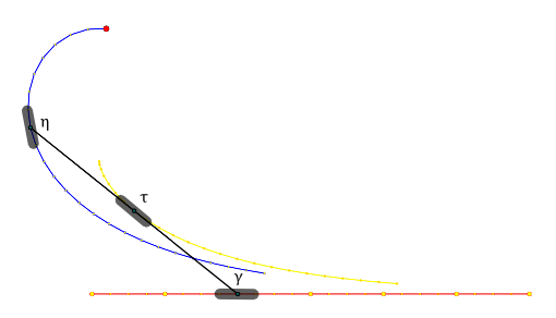
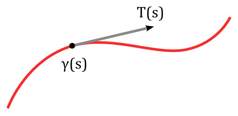
Let us investigate the tracks traced out by the wheels of a moving bicycle during some time interval $[a,b]$. We denote the path of the (center of the) rear wheel  by $\tau$ and the path of the front wheel by $\gamma$. If $\ell$ is the distance between the rear and the front wheel then at each time $t$ the direction of the bicycle is given by a unit vector $T(t)$ such that

\[\gamma=\tau+\ell\, T.\]

In the picture below the front wheel $\gamma$ moves on a straight line. The resulting path of the rear wheel is called the tractrix curve and has been investigated already in 1676 by Isaac Newton and in 1692 by Christian Huygens.

 

Assuming that the rear wheel rolls without sliding it must move in the direction of $T$: There is a function $\rho: [a,b] \to \mathbb{R}$ such that

\[\tau’=\rho T.\]

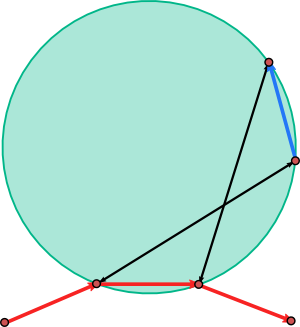
Suppose the bicycle is prolonged in the rear direction by a rod. We assume that the tip of the rod has distance $\ell$ to the center of the rear wheel (only projections to the horizontal plane are considered here). Then the position $\eta(t)$ of the tip of the rod is given as

\[\eta=\tau-\ell T.\]

The rotation speed $\omega(t)$ of the bicycle is defined via

\[T’=\omega JT.\]

From

\begin{align*}\gamma’ &= \rho’ T+\ell \omega JT \\\\ \eta’ &= \rho’ T-\ell \omega JT \end{align*}

it is easy to see that the velocity vector $\eta’$ of the back end is equal in magnitude to the speed $\gamma’$ of the front wheel:

\[|\eta’|^2=\rho’^2+\omega^2=|\gamma’|^2.\]

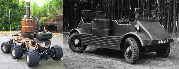
Moreover, if we were to install another wheel at the rear end that also rolls without sliding it would have to make the same angle (though opposite in direction) with the bicycle as the front wheel. Such a bicycle (omitting the middle wheel) has in fact been built, even though I have to admit that the video does not look convincing.

On the other hand, cars with four-wheel steering are manufactured in some variety. The motion of cars with four wheels is more difficult to analyze, but to some approximation we might assume also here that the center $\tau$ of the rear axis moves towards the center $\gamma$ of the front axis. The right picture below shows a DAF MC-139 prototype from 1940 (yes, it has two driver seats). The model in the left picture even has the middle wheels (showing the tractrix) and a video can be found here.

Let us condense all this into a mathematical

Definition: Let $\tau: [a,b]\to \mathbb{R}^n$ be a path and suppose there are $T:[a,b] \to\mathbb{R}^n$ of unit length $|T|=1$ and $\rho: [a,b] \to \mathbb{R}$ such that $\tau’=\rho T$. Then for every $\ell\in \mathbb{R}$ the path $\tau$ is called a tractrix of the path $\gamma:=\tau+\ell\,T$. Furthermore $\eta:=\tau-\ell\,T$ is called a Darboux transform of $\gamma$.

It is easy to see that in the above situation $\tau$ is a tractrix also of $\eta$ and $\gamma$ also is a Darboux transform of $\eta$. The paths $\gamma$ and $\eta$ always have the same length. Note that if $\gamma$ is regular then so is $\eta$ and if $\gamma$ is parametrized by arclength then the same holds for $\eta$.

We can apply similar definitions in the case of closed curves by assuming that $\tau$, $T$ and $\rho$ are periodic functions.

Theorem: Suppose $\eta$ is a Darboux transform of a periodic path $\gamma$ in $\mathbb{R}^n$ that is parametrized by arc length. Then $\gamma$ and $\eta$ have the same length and the same total squared curvature

\[\oint |\gamma”|^2=\oint |\eta”|^2.\]

If $n=3$ then $\gamma$ and $\eta$ have the same area vector

\[\frac{1}{2}\oint \gamma \times \gamma’ = \frac{1}{2}\oint \eta \times \eta’.\]

Proof: We have

\[\gamma’=\rho T + \ell T’\]

and we may assume that $\gamma$ and $\eta$ are parametrized by arc length, i.e.

\[\rho^2+\ell^2|T’|^2=1.\]

Then

\[\gamma”=\rho’T+\rho T’+\ell T”\]

and

\[\oint \langle \gamma”,\gamma”\rangle =\oint \rho’^2 + 2\ell \langle \rho’ T +\rho T’,T”\rangle +\ell^2 |T”|^2.\]

We want to show that this expression is unchanged if we replace $\ell$ by $-\ell$, i.e.

\[\oint  \langle \rho’ T +\rho T’,T”\rangle = \oint -\rho’ \langle T’,T’ \rangle – \frac{\rho}{2}\langle T’,T’\rangle’ =\oint  \rho'(\rho^2-1)+\rho^2\rho’=0.\]

Here we have used $0=\langle T,T’\rangle’=\langle T’,T’\rangle+\langle T,T”\rangle$, the equation $\rho^2+\langle T’,T’\rangle =1$ and its derivative $2\rho \rho’+\langle T’,T’\rangle’=0$.

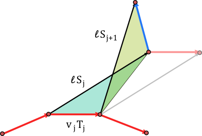
Next we look at the area vector

\[\oint \gamma \times \gamma’ = \oint (\tau+\ell T)\times (\rho T+\ell T’).\]

Again we only have to show that the coefficient of $\ell$ vanishes, i.e.

\[\oint \tau \times \ell T’ = \oint (\tau \times \ell T)’=0.\]

$\square$

The statement about the area vector implies for the case $n=2$ that $\gamma$ and $\eta$ enclose the same area:

\[\frac{1}{2}\oint \mbox{det}(\gamma, \gamma’) = \frac{1}{2}\oint \mbox{det}(\eta,\eta’).\]

 

A path in $\mathbb{R}^n$ is a $C^\infty$ map

\[\gamma: [a,b] \to \mathbb{R}^n.\]

We imagine $\gamma$ as the path traced out by a moving point $\gamma(t)\in \mathbb{R}^n$ over the time interval $[a,b]$. Such a path $\gamma$ is called regular if $\gamma'(t) \neq 0$ for all $t\in [a,b]$. Suppose we have another path $\tilde{\gamma}: [\tilde{a},\tilde{b}] \to \mathbb{R}^2$ that reaches every point $\gamma(t)$ covered by $\gamma$, only at a different time $\tilde{t}=\varphi(t)$. Thus we have

\[\tilde{\gamma}=\gamma \circ \varphi.\]

We assume that $\varphi$ is $C^\infty$ and maps the interval $[\tilde{a},\tilde{b}]$ diffeomorphically onto $[a,b]$ in an orientation-preserving fashion:

\begin{align*}\varphi(\tilde{a})&=a \\ \varphi(\tilde{b})&=b \\ \varphi’ &>0.\end{align*}

Then we say that $\tilde{\gamma}$ is just a reparametrized version of the same “curve segment”. Thus curve segments are defined as equivalence classes of planar paths. Note that the reversed path

\begin{align*}\tilde{\gamma}:[a,b] &\to \mathbb{R}^2 \\ \tilde{\gamma}(t)&=\gamma(b+a-t)\end{align*}

in general defines a different curve segment. Thus curve segments come with a well defined orientation. They have a definite starting point.

Fortunately, we almost never have to deal with issues of reparametrization. This is because every curve segment has a canonical parametrization, its so-called parametrization by arc length: For a regular path $\gamma:[a,b]\to\mathbb{R}^n$ its length is defined as

\[\mbox{length}(\gamma)= \int_a^b |\gamma’|.\]

Then with the notation $L:=\mbox{length}(\gamma)$ the function

\begin{align*}\ell:[a,b] &\to [0,L] \\ \ell(t)&=\mbox{length}(\gamma|_{[a,t]})\end{align*}

has a smooth inverse $\varphi:[0,L] \to [a,b]$ and $\tilde{\gamma}=\gamma\circ\varphi$ has a velocity vector field $T=\tilde{\gamma}’$ of unit length:

\[|\tilde{\gamma}’|=1.\]

Any path with this property is called an arc length parametrization of a curve in $\mathbb{R}^n$.

A periodic path in $\mathbb{R}^n$ is a pair $(\gamma,\tau)$ where $\gamma: \mathbb{R} \to \mathbb{R}^n$ is $C^\infty$ and $\tau$-periodic, which means that for all $t\in \mathbb{R}$ we have

\[\gamma(t+\tau)=\gamma(t).\]

Again, such a closed path is called regular if $\gamma'(t) \neq 0$ for all $t\in\mathbb{R}$. A smooth map $\varphi: \mathbb{R} \to \mathbb{R}$ such that

\begin{align*}\varphi’&>0\\ \varphi(\tilde{t}+\tilde{\tau})&=\varphi(\tilde{\tau})+\tau\end{align*}

defines a reparametrization $(\tilde{\gamma},\tilde{\tau})$ of $(\gamma,\tau)$. A closed curve in $\mathbb{R}^n$ is an equivalence class of periodic paths with respect to reparametrization.

 

The length of a closed curve $(\gamma,\tau)$ is defined as the length of the path $\gamma|_{[0,\tau]}$. If $L$ is the length of a regular periodic path $(\gamma,\tau)$ then one  can show as before that there is a reparametrization $(\tilde{\gamma},L)$ with $|\tilde{\gamma}’|=1$. Note however that such an arc length parametrization of a regular closed curve is unique only up to a parameter translation: For every $a\in \mathbb{R}$ the periodic path $s\mapsto \hat{\gamma}(s)=\tilde{\gamma}(s+a)$ has the same property.