Let us first look at the smooth case. Let $\gamma\colon I\to \mathbb{R}^3$ be an arc length parameterized smooth curve with tangent vector $T:=\gamma^\prime$.

An adapted frame is then a smooth map $\sigma\colon I\to SO(3)$ such that $\sigma e_1 = T$. We denote the second and the third column of $\sigma$ by $N$ and $B$ $$\sigma= (T,N,B).$$ The fields $N$ and $B$ are normal vector fields. Clearly $B=T \times N$.

Let us take the derivative of $\sigma$. Since the vectors $T,N,B$ are normalized we find that $$\sigma^\prime=\sigma \mathcal{U},$$ where $$\mathcal{U}=\begin{pmatrix}0 & \kappa_1 & \kappa_2 \\ -\kappa_1 & 0 & -\tau \\ -\kappa_2 & \tau & 0 \end{pmatrix}.$$

If $N$ is parallel along $\gamma$, i.e. the derivative has only a tangential component $N^\prime= \kappa_1 T$, then so is $B$, and $\tau$ vanishes: $$\mathcal{U}=\begin{pmatrix}0 & \kappa_1 & \kappa_2 \\ -\kappa_1 & 0 & 0 \\ -\kappa_2 & 0 & 0 \end{pmatrix}.$$ Such a frame is called a parallel frame. We have seen in the lecture that parallel frames always exist.

If $\sigma=(T,N,B)$ is a parallel frame and $\alpha\in\mathbb{R}$, then we define a new frame $\sigma_\alpha= (T,N_\alpha,B_\alpha)$ with $$N_\alpha = \cos\alpha\, N+ \sin\alpha\, B,\quad B_\alpha=-\sin\alpha\, N+ \cos\alpha\, B.$$ This frame is parallel again.

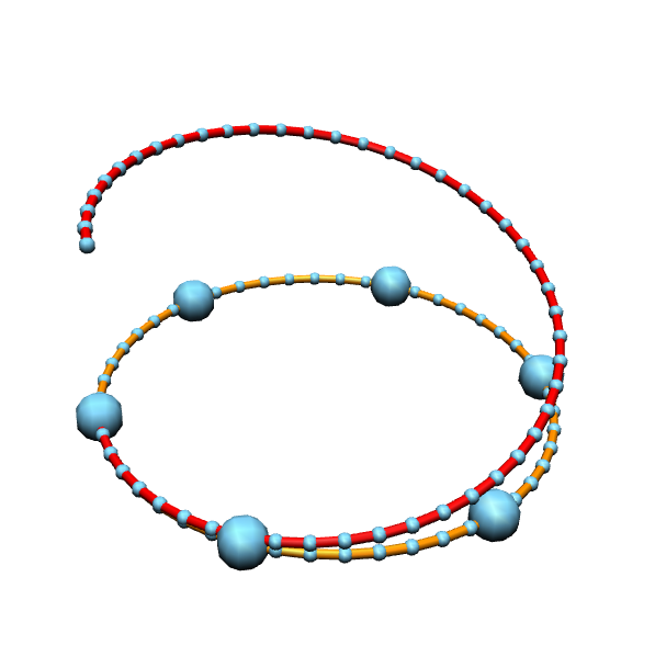
The point now is that, up to Euclidean motion, $\gamma$ is determined by $\mathcal{U}$. We can just solve for $\sigma$ and obtain $T$ as its first column. The curve is then reconstructed by integrating $T$.

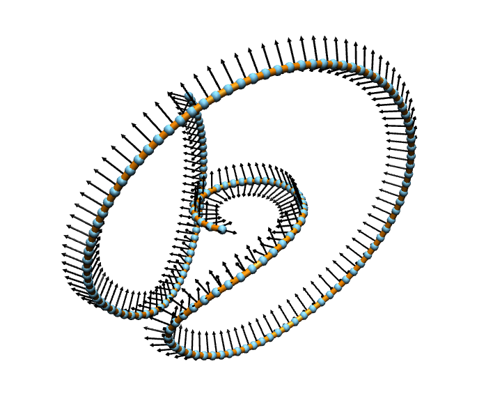
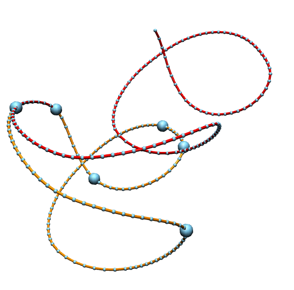
The term spinning refers then to the following procedure. We start with a curve $\gamma$ and a parallel frame $\sigma$. This gives us $\mathcal{U}$ with $\kappa_1$ and $\kappa_2$. Now we define $\mathcal{U}_\lambda$ for $\lambda\in\mathbb{R}$ as follows $$\mathcal{U}_\lambda=\begin{pmatrix}0 & \kappa_1 & \kappa_2 \\ -\kappa_1 & 0 & -\lambda \\ -\kappa_2 & \lambda & 0 \end{pmatrix}.$$ This determines a new curve $\gamma_\lambda$. This family of curves is called the associated family.

  

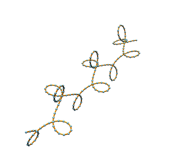
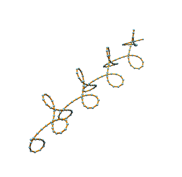
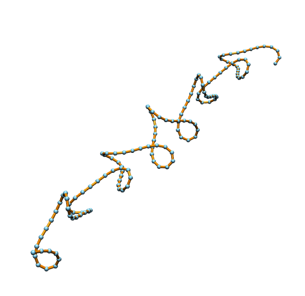
Our plan is to spin discrete space curves. So let $\gamma=(\gamma_0,\dots,\gamma_n)$ be a discrete space curve. Thinking of linear interpolation one finds the best place to locate an adapted frame is on the edges. Here it is clear what the tangent $T_i$ shall be $$\gamma_i^\prime:=\gamma_{i+1}-\gamma_i= \ell_i T_i.$$

Since the tangent on each edge is constant, we can put just a constant frame on each edge, i.e. for each edge we get $\sigma_i$ such that $\sigma_i e_1= T_i$. Only at vertices the frame field has to jump.

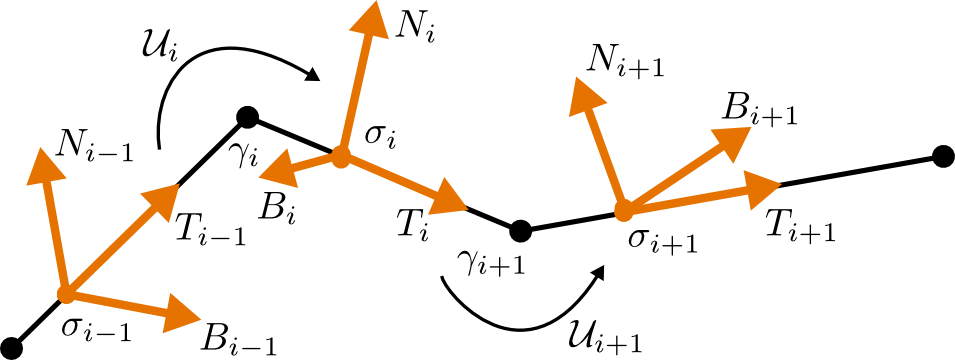
We define a discrete adapted frame as a collection of $SO(3)$-matrices $\sigma_i$ such that $\sigma_i e_1= T_i$.

The jumps over the vertices are again given by $SO(3)$-matrices $\mathcal{U}_i$, which we will call transport matrices. Quiet analogue to the smooth we have $$\sigma_i= \sigma_{i-1} \mathcal{U}_i.$$

As in the smooth world the transport matrices determine the adapted frame. If a initial value $\sigma_0$ is given then $\sigma_i$ is given by $$\sigma_i=\sigma_0\mathcal{U}_1 \cdots\mathcal{U}_i.$$

The corresponding curve is then reconstructed by integration of $T= \sigma e_1$. So we get for $\gamma_0\in \mathbb{R}^3$ and $\sigma_0$: $$\gamma_{k+1} = \gamma_0 + \sigma_0 \bigl(\sum_{i=0}^k \ell_i\mathcal{U}_1 \cdots\mathcal{U}_i\bigr)e_1.$$

Again we find special transport matrices, namely these which change the frame as minimal as possible, i.e. if $T_{i-1}$ and $T_i$ are parallel then $\mathcal{U}_i=Id$ and else $\mathcal{U}_i$ rotates $\sigma_{i-1}$ around $T_{i-1}\times T_i$. These transport matrices we will denote by parallel transport. They come directly with the geometry of the curve.

A frame with such transport matrices is called a discrete parallel frame. Each discrete curve admits a parallel frame.

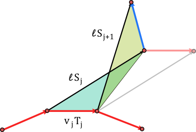
Now let $\gamma$ be a discrete space curve with a parallel frame $\sigma=(T,N,B)$. Then this defines complex numbers $q$ at the vertices in the following way: Consider the vertex $\gamma_{i+1}$. The plane $\mathcal{N}_{i}$ spanned by the vectors $N_{i},B_{i}$ can be considered as complex line with rotation given by 90-degree-rotation around $T_{i}$ which we will denote by $J$, i.e. $JX=T_i\times X$. The next tangent vector $T_{i+1}$ lies on the unit sphere with the point $-T_{i}$ removed.

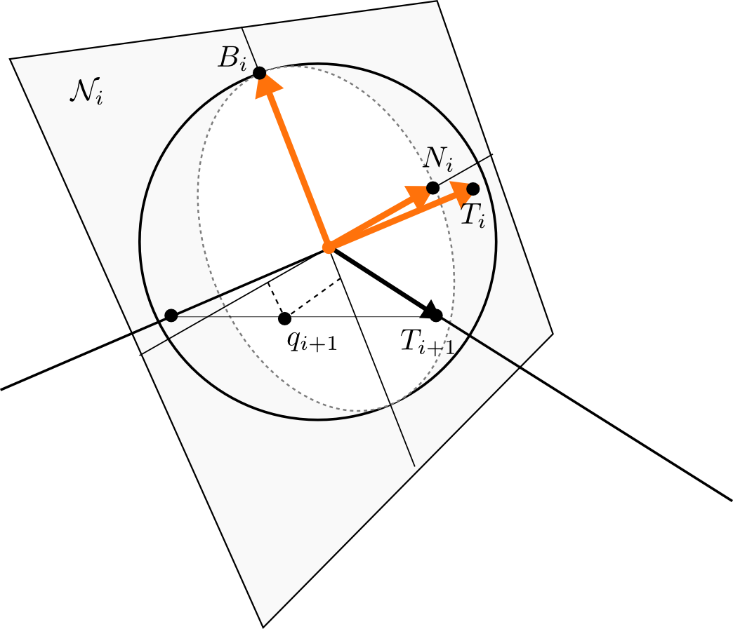
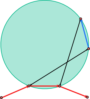
If we perform stereographic projection with respect to the north pole $-T_{i}$, then the tangent vector $T_{i+1}$ is mapped to $\mathcal{N}_i$ and hence defines a complex number $$q_{i+1}=\kappa_1\, N_i + \kappa_2 B_i=(\kappa_1 + \kappa_2 J) N_i.$$ This can be interpreted as discrete complex curvature.

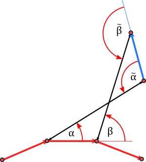
If the tangents are linearly dependent then $q=0$. If they are not they span a plane. We slice the sphere by this plane and find that the magnitude of $q$ is given by $$|q|= \tan(\tfrac{\alpha}{2}),$$ where $\alpha$ is the angle between $T_i$ and $T_{i+1}$.

In general frames can have torsion. While the curvature is located at the vertices, we define the torsion on the edges. Let $\sigma$ be an arbitrary frame. Imagine the frames located at the start of the edges. We want to know how much it rotates around the edge from the beginning to the end. To get the rotation angle we use the parallel transport to pull the frame on the next edge back to the end of the current. I.e. we have $\sigma_i$ and $\sigma_{i+1}\mathcal{U}_{i+1}^{-1}$, both adapted to the i-th edge. They differ by a rotation around $T_i$. If $\alpha$ is the angle of the rotation, then the torsion $\tau_i$ is given by $$\alpha= \tau_i \ell_i.$$

To go further, we change to quaternionic frames in which the transports takes a much simpler form. Therefore we identify $\mathbb{R}^3$ with the imaginary quaternions, i.e. $$x_1e_1+x_2e_2+x_3e_3 \longleftrightarrow x_1\mathbf{i}+ x_2\mathbf{j}+x_3\mathbf{k}.$$ With this identification a rotation around an axis given by a vector $X$ with $|X|=1$ by an angle $\alpha$ takes the form $$P\mapsto X_\alpha PX_\alpha^{-1},$$ where $$X_\alpha=\cos(\alpha/2)\mathbf{1} +\sin(\alpha/2)X.$$

So we can encode the frame equations by quaternions by considering $\phi_i$ such that $$T_i = \phi_i\, \mathbf{i}\,\phi_i^{-1},\quad N_i = \phi_i\, \mathbf{j}\,\phi_i^{-1},\quad B_i = \phi_i\, \mathbf{k}\,\phi_i^{-1}.$$ That is $\phi$ rotates the standard basis to the basis given by the frame $\sigma_i$. By the equations above $\phi_i$ is determined up to a non-zero scale factor. As before the frames $\phi_i$ are related by transports, i.e. $$\phi_{i}=\phi_{i-1}\mathcal{V}_i.$$

The reconstruction formula for the corresponding curve takes a quite similar form $$\gamma_{k+1}= \gamma_0 + \phi_0\bigl( \sum_{i=0}^{k}\ell_i (\mathcal{V}_1\cdots \mathcal{V}_i )\,\mathbf{i}\, (\mathcal{V}_1\cdots \mathcal{V}_i)^{-1}\bigr)\phi_0^{-1}.$$

Once we know the $q$ the parallel transport takes an amazingly simple for in the quaternionic setting. It is given by $$\mathcal{V}_i = \mathbf{1}+ \mathbf{i}q\mathbf{j}= \mathbf{1}+ q\mathbf{k}= \mathbf{1} -\operatorname{Im}(q)\mathbf{j}+\operatorname{Re}(q)\mathbf{k}.$$

This is due to the fact that $-\operatorname{Im}(q)\mathbf{j}+\operatorname{Re}(q)\mathbf{k}$ are the coordinates (wrt. $\phi_{i-1}$) of the rotation axis prescribed by parallel transport and $|q|=\tan(\alpha/2)$, where $\alpha$ is the rotation angle.

The rotation around the tangent takes the simple form $\mathcal{T}_i^\alpha=\cos(\alpha\ell_i)\mathbf{1}+\sin(\alpha\ell_i)\mathbf{i}$. Hence we can spin the curve in the following way:

1. Take a parallel frame and calculate the corresponding $q$’s.
2. Define for $\lambda\in \mathbb{R}$ a new parallel transport by $\mathcal{V}^\lambda_i=\mathcal{T}^\lambda_{i-1}\mathcal{V}_i$.
3. Reconstruct the curve corresponding the $\mathcal{V}^\alpha_i$.

 

Homework (due date 27 June): Your task is to implement the spinning procedure, i.e. write a plugin the constructs for a given $\lambda\in\mathbb{R}$ the curve corresponding to the transports $\mathcal{V}^\lambda_i$ as define above and adds it to the scene. The initial values should be chosen suitably.

As in the last post let $\gamma$ be a discrete curve in the $\mathbb{C}$ and $\tilde{\gamma}= \gamma+ \ell S$ be a Darboux transformation. Denote by $\alpha_j$ and $\beta_j$ the angles from the edges $T_J$ of $\gamma$ to the rod directions $S_j$ and $S_{j+1} respectively. Then

$$\begin{align*}S_j &= e^{i \alpha_j} T_j \\\\ S_{j+1}&= e^{i \beta_j} T_j.\end{align*}$$

We know that $S$ satisfies

$$S_{j+1}=\frac{\ell S_j- v_j T_j}{\ell-v_j \bar{T}_j S_j}.$$

This yields

$$e^{i\beta_j}=\frac{\ell e^{i\alpha_j}- v_j}{\ell-v_j e^{i\alpha_j}}.$$

Using the formula

$$e^{i\alpha}=\frac{1+it}{1-it}$$

where

$$t:=\tan \frac{\alpha}{2}$$

we then have

$$\begin{align*} e^{i\beta_j}&=\left(\ell \frac{1+it_j}{1-it_j}- v_j \right) \left(\ell-v_j \frac{1+it_j}{1-it_j} \right)^{-1} \\\\ &=\left(\frac{(\ell -v_j)+(\ell +v_j)it_j}{1-it_j}\right) \left( \frac{(\ell-v_j )-(\ell+v_j )it_j}{1-it_j} \right)^{-1} \\\\ &= \frac{1+i \mu_j t_j}{1-i \mu_j t_j} \,.\end{align*}$$

where

$$\mu_j= \frac{\ell+v_j}{\ell-v_j}.$$

From this we conclude

$$\tan \frac{\beta_j}{2}=\mu_j \tan \frac{\alpha_j}{2}.$$

With the notation

$$\begin{align*}t_j&:=\tan \frac{\alpha_j}{2}\\\\ \tau_j&:=\tan \frac{\kappa_j}{2}\end{align*}$$

we obtain

$$\begin{align*}\tau_j&=\tan \frac{\beta_{j-1}-\alpha_j}{2}\\\\ &= \frac{\mu_{j-1} t_{j-1}-t_j}{1+\mu_{j-1} t_{j-1} t_j}.\end{align*}$$

The corresponding quantities for the Darboux transform $\tilde{\gamma}$ are

$$\begin{align*}\tilde{\alpha}_j &=\pi-\beta_j \\\\ \tilde{\beta}_j &= \pi- \alpha_j \\\\ \tilde{\tau}_j&=\tan \frac{\beta_j-\alpha_{j-1}}{2}\\\\ &= \frac{\mu_j t_j-t_{j-1}}{1+\mu_j t_j t_{j-1}}.\end{align*}$$

Note that we arrive at $\tilde{\tau}_j$ starting from $\tau_j$ if we interchange the roles of $t_{j-1}$ and $t_j$ and replace $\mu_{j-1}$ by $\mu_j$. If we apply this rule to

$$\begin{align*}1+\tau_j^2 &= \frac{(1+2\mu_{j-1} t_{j-1} t_j +\mu_{j-1}^2 t_{j-1}^2 t_j^2) + (t_j^2 -2 \mu_{j-1} t_{j-1} t_j +\mu_{j-1}^2 t_{j-1}^2)}{(1+\mu_{j-1} t_{j-1} t_j)^2} \\\\ &= \frac{(1+t_j^2)(1+\mu_{j-1}^2 t_{j-1}^2)}{(1+\mu_{j-1} t_{j-1} t_j)^2} \end{align*}$$

we obtain

$$1+\tilde{\tau}_j^2=\frac{(1+t_{j-1}^2)(1+\mu_j^2 t_j^2)}{(1+\mu_j t_j t_{j-1})^2}$$

Now the following is easy to prove:

Theorem: If $\gamma$ is a closed polygon in $\mathbb{R}^2$ with equal edge lengths and $\tilde{\gamma}$ is a closed Darboux transform of $\gamma$ then

$$\prod_{j=1}^n (1+\tau^2) = \prod_{j=1}^n (1+\tilde{\tau}^2).$$

We can interpret this as follows: The bending energy

$$\sum_{j=1}^n \log (1+\tau_j^2)=-\sum_{j=1}^n \log (1+\cos \kappa_j)$$

is the same for $\gamma$ and $\tilde{\gamma}$.