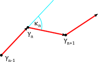
As we saw in the  lecture, we can parametrize the moduli space of discrete closed plane curves by angles and edge lengths, which encode how the tangent is moving along the curve. More explicit: up to rigid motion each discrete curve with \(n\) vertices and tangent winding number \(m\) is represented by a point in a submanifold \(\mathcal{M}_0\) of \((-\pi,\pi)^{n}\times (0,\infty)^{n}\), which is given by the zero set of the map \[ F:(-\pi,\pi)^{n}\times (0,\infty)^{n} \to \mathbb{R}^3 = \mathbb{R}\times \mathbb{C}\\\\ F(\ell,\kappa)=\left(\begin{array}{c} \kappa_1+\ldots +\kappa_n -2 \pi m \\  \ell_1 e^{i\alpha_1}+\ldots +\ell_{n}\, e^{i\alpha_{n}}\end{array}\right),\] where \[\alpha_j= \kappa_1+\ldots+\kappa_j.\]

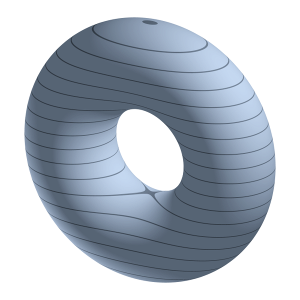
In general, each function defined on \(\mathcal{M}\) splits the space into components. E.g. think  of a height function of an embedded surface.

If the map is ‘nice’ enough, i.e. in our case smooth and of constant rank, then the level sets are submanifold. Moreover \(\mathcal{M}_0\) is the intersection of the submanifolds \(\mathcal{M}_1\) and \(\mathcal{M}_2\), which are given as zeros sets of the functions\[F_1(\ell,\kappa)=\kappa_1+\ldots +\kappa_n -2 \pi m, \quad F_2(\ell,\kappa)=\ell_1 e^{i\alpha_1}+\ldots +\ell_{n}\, e^{i\alpha_{n}}.\]

Now, we have given \(\mathcal{M}_0\) which parameterizes discrete closed plane curves. But what does the ambient space correspond to?

It is important to note that a closed curve is in fact rather a periodic sequence of points than just \(n\) points. With this in mind, let us assign to each point in \((-\pi,\pi)^{n}\times (0,\infty)^{n}\) periodic sequences, denoted again by \(\kappa\) and \(\ell\), to which corresponds a discrete curve \(\gamma \colon \mathbb{Z}\to \mathbb{C}\). The curve \(\gamma\) is obtain by ‘integration’, i.e. e.g. for positive \(k\) we have\[\gamma_{k+1}=\sum_{j=1}^k \ell_j e^{i\alpha_j}.\]

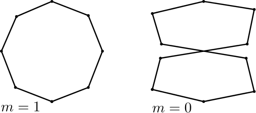
Now we can directly look at the effect of dropping conditions: Let us start outgoing from the case that \(\kappa,\ell\) lies on \(\mathcal{M}_0\), i.e. we have a discrete closed plane curve as shown below.

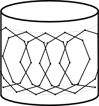
If we drop the second condition we just stay on \(\mathcal{M}_1\), i.e. the curves do not have to close up but the tangent winding number is still restricted to \(2\pi m\), such curves are know as curves with translational period. Examples are shown below.

These curves can also regarded as closed curves on a cylider.

Our task is now to navigate on the submanifold \(\mathcal{M_0}\), i.e. given a vector field \(X\) on \(\mathcal{M_0}\) and a point \(p \in\mathcal{M_0}\), then move along the integral curve of \(X\) starting at \(p\).

In our setup we are surrounded by a Euclidean space that means that tangent vector fields are just maps into \(\mathbb{R}^{2n}\). First, let us ignore all conditions for a moment. Then we can just use the Euler method to follow the vector field, i.e. we just go a bit in the direction of the vector field: If at time \(t\) we are at the position \(p(t)\), then \[ p(t+\varepsilon)= p(t)+\varepsilon X(p(t)),\] is the position at time \(t+\varepsilon\). Since this shall correspond to a discrete curve that was obtained by regular homotopy we have to ensure that we don’t leave the open subset \((-\pi,\pi)^{n}\times (0,\infty)^{n}\). But that’s easy.

It is also easy to stay in \(\mathcal{M}_1\) as it consists of open subsets of affine vector spaces, i.e. all one has to do is to project the given vector field \(X\) to the tangent space of \(\mathcal{M}_1\). If \(X^\top\) denotes the projection, the corresponding line \(p+\operatorname{span}\{X^\top(p)\}\) is then already contained in the affine vector space. Again all we have to ensure is that the point does not leave an open set.

The situation changes if we start at a closed curve \(p(t)\) and want to stay closed. First, the vector field then has to be tangential to \(\mathcal{M}_0\), i.e. we have to eliminate the normal components. Second, even if the field is tangential, we will leave \(\mathcal{M_0}\) Immediately if we move along a line. Our strategy will be to fix this by projecting back to \(\mathcal{M_0}\) after each Euler step.

Let us focus on the situation that all lengths shall stay fixed during the flow as it was presented in the lecture, i.e. all components of the vector field that correspond to lengths are just zero:\[X(p)=(X_1(p),\dots,X_{n}(p),0,\dots,0).\]

The normal space to \(\mathcal{M}_0\) at a point \(p=(\kappa_1,…,\kappa_{n},\ell_0,…,\ell_{n}) \in \mathcal{M}_0\) was spanned by \[V_0=(1,\dots,1,0,\dots,0)\] and the vertex coordinates of a curve \(\gamma\) corresponding to the point \(p\) \[ V_1=(x_1,\dots,x_j,0,\dots,0),\\ V_2=(y_1,\dots,y_j,0,\dots,0),\] where the \(x_j\) and \(y_j\) denotes the real and imaginary part of \(\gamma_j\) resp., i.e. \(\gamma_j=x_j+iy_j\).

We apply the Gram-Schmidt process starting with \(V_0\) and obtain an orthonormal basis \(N_0,N_1,N_2\) of the normal space of \(\mathcal{M}_0\). The projection of \(X\) on its tangential part \(X^T\) then takes the simple form\[X^\top=X-\sum_{j=0}^2\langle X,N_j\rangle N_j.\]

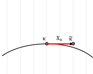
We perform the Euler step with respect to the field \(X^\top\) and obtain a new point \(\tilde p=(\tilde\kappa,\ell)\) which a priori not yields a closed curve. Now we have to get back to \(\mathcal{M}_0\), i.e. we have to change the \(\tilde\kappa\) slightly so that \(F(\tilde\kappa,\ell)=0\). Hence we have to search for a zero of a non-linear function in an \(n\)-dimensional space, which in general is slow and the speed moreover depends on the number of vertices.

We reduce this problem, as proposed, to a \(2\)-dimensional one by projecting \(\tilde p\) back along the normal space at the previous point \(p\):\[f(\lambda_1,\lambda_2)=F(\tilde\kappa+\lambda_1N_1+\lambda_2 N_2,\ell)=0.\]

This we solve by applying the Newton method and obtain a new closed curve.

Homework (due date 6 June): Your task is to implement the gradient flow of the bending energy on closed curves. In the repository you find under de.jtem.discreteCurves.tutorial a class called GradientFlowPlugin which provides a basic environment to start with. It shows the gradient flow of the bending energy\[E(\kappa,\ell)= \tfrac{1}{2}\sum_{j=1}^{n} \kappa_j^2.\] without any constraints, i.e. closed curves immediately open up and are deformed into straight lines.

Copy the GradientFlowPlugin into your project.

Your task is now to modify the flow so that closed curves stay closed, i.e. you have the following things to do:

1. Project the gradient of the bending energy to the tangent space of \(\mathcal{M}_0\) to obtain a vector field \(X\) which is tangential.
2. Implement the projection back to \(\mathcal{M}_0\) after the Euler step.

The Euler step just stays as it is. For the second item you can use the Newton method that is implemented in the jtem project numericalMethods (explicitly in de.jtem.numericalMethods.calculus.rootFinding).

Hint: Even if it is not an example for the usage of the Newton-class it may be helpful to look into ExampleNewtonRaphson, which you find at the same place.

In this post we will work with a fixed sequence of lengths  $\ell_1,\dots,\ell_n>0$. This means we imagine polygons as composed of rigid edges connected by flexible joints at the vertices. Denote by $\mathcal{M}_m$ the space of curvature functions $\kappa=(\kappa_1,\ldots,\kappa_n)$ that correspond to closed regular polygons with $n$ vertices and tangent winding number $m$.  We can conveniently describe $\mathcal{M}_m$ as the zero set of the function

\begin{align*}\qquad F:(-\pi,\pi)^n &\to \mathbb{R}^3 = \mathbb{R}\times \mathbb{C}\\\\ F(\kappa_1,\ldots,\kappa_n)&=\left(\begin{array}{c} \kappa_1+\ldots +\kappa_n -2 \pi n \\  \ell_0 e^{i\alpha_0}+\ldots +\ell_{n-1}\, e^{i\alpha_{n-1}}\end{array}\right).\end{align*}

By the above calculation the derivative of $F$ is given as

\[F'(\kappa_1,\ldots,\kappa_n)\left(\begin{array}{c}\dot{\kappa}_1\\ \vdots \\ \dot{\kappa}_n\end{array}\right)=\left(\begin{array}{c} \dot{\kappa}_1+\ldots +\dot{\kappa}_n \\ \dot{\kappa}_1 \gamma_1+\ldots + \dot{\kappa}_n \gamma_n \end{array}\right).\]

Theorem: The rank of $F’$ is three at all points of $\mathcal{M}_m$. Therefore, by the implicit function theorem, $\mathcal{M}_m$ is a smooth manifold.

Proof: At a point $(\kappa_1,\ldots,\kappa_n)$ where the columns of $dF(\kappa_1,\ldots,\kappa_n)$ were linearly dependent we would have $a,b,c\in \mathbb{R}$ such that

\[a \mbox{Re}(\gamma_j)+b \mbox{Im}(\gamma_j)+c=0\]

for all $j$. But this means that the whole polygon lies on a straight line, which is impossible for a regular polygon.

$\square$

Suppose we have a vector field tangent to $\mathcal{M}_m$ that we want to follow numerically. This means that for any $\kappa=(\kappa_1,\ldots,\kappa_n)\in \mathcal{M}_m$  we are given a certain tangent vector

\[X_\kappa \in T_\kappa \mathcal{M}_m=\mbox{ker}F'(\kappa).\]

We want to find curves $t\mapsto \eta(t)\in \mathcal{M}_m$ that satisfy for all $t$

\[\dot{\eta}(t)=X_\eta(t).\]

If we already have constructed $\kappa=\eta(t)$ we might attempt to find $\eta(t+\epsilon)$ as

\[\tilde{\kappa}=\kappa+\epsilon \dot{\kappa}\]

where $\dot{\kappa}=X_{\kappa(t)}$. Since $\dot{\kappa}$ lies in the kernel of $F'(\kappa)$ the condition

\[\tilde{\kappa}_1+\ldots+\tilde{\kappa}_n=2\pi m\]

will be satisfied. The second condition

\[\ell_0 e^{i\tilde{\alpha}_0}+\ldots +\ell_{n-1} \,e^{i\tilde{\alpha}_{n-1}}\]

however is non-linear and so we cannot be sure that $\tilde{\kappa}$ corresponds to a closed regular polygon. We first have to project $\tilde{\kappa}$ back to $\mathcal{M}_m$.

To this end we add to $\tilde{\kappa}$ an element of $(T_\kappa\mathcal{M}_m)^\perp$, the normal space to $\mathcal{M}_m$ at the point $\kappa$. This space is spanned by

\begin{align*}N_0&=(1,\ldots,1)\\\\ N_1&=(x_1,\ldots,x_n) \\\\ N_2 &=(y_1,\ldots,y_n)\end{align*}

Here $\gamma_j=x_j+iy_j$ and we assume that a translation has been applied to $\gamma$ in order to achieve

\[\gamma_1+\ldots,+\gamma_n=0.\]

Since the condition $\tilde{\kappa}_1+\ldots+\tilde{\kappa}_n=2\pi m$ already has been dealt with there is no need to work with $N_1$. We therefore are looking for $\lambda_1,\lambda_2 \in \mathbb{R}$ such that

\[f(\lambda_1,\lambda_2)=(0,0).\]

Here

\[f(\lambda_1,\lambda_2)=G(\kappa+\lambda_1 N_1 + \lambda_2 N_2)\]

where

\[G(\hat{\kappa}):=\ell_1e^{i\hat{\alpha}_1}+\ldots+\ell_{n-1}e^{i\hat{\alpha}_{n-1}}\,.\]

Thus we are left with the problem of finding a zero of $f$. From the calculation at the beginning of the post we know the derivative of $f$, so a Newton method seems the right thing to implement.

The moduli space (meaning congruent polygons are considered as equal) of open regular polygons $\gamma_0,\ldots,\gamma_n$ in the plane can be parametrized by parameters

\[(\ell_0,\ldots,\ell_{n-1},\kappa_1,\ldots,\kappa_{n-1})\in (0,\infty)^{n-1} \times (-\pi,\pi)^{n-2}.\]

If we we want to construct an actual polygon from such data we first define $\alpha_0,\ldots,\alpha_{n-1}$ as

\[\alpha_j=\kappa_1+\ldots+\kappa_j.\]

From these we define normalized edge vectors $T_j=e^{i\alpha_j}$ and finally the polygon itself: For $j=0,\ldots,n$ we set

\[\gamma_j=\ell_0 T_0+\ldots+\ell_{j-1} T_{j-1}.\]

The direction of the edge joining $\gamma_j$ to $\gamma_{j+1}$ is given by $T_j=e^{i\alpha_j}$ with . Then the position $\gamma_n$ of the last vertex (equal to $\gamma_0$ for a closed polygon) is given a

\[\gamma_n=\ell_0 e^{i\alpha_0}+\ldots +\ell_{n-1} e^{i\alpha_{n-1}}.\]

Theorem (Schläfli Formula): From given parameters

\[(\ell_0,\dots,\ell_{n-1},\kappa_1,\ldots,\kappa_{n-1})\in (0,\infty)^{n-1} \times (-\pi,\pi)^{n-2}\]

construct a polygon $\gamma_0,\ldots,\gamma_n$ as described above. Consider a variation $(\dot{\ell}_0,\dots,\dot{\ell}_{n-1},\dot{\kappa}_1,\ldots,\dot{\kappa}_{n-1})$ of these parameters and define

\[\dot{\kappa}_n:=-(\dot{\kappa}_1+\ldots+\kappa_{n-1}).\]

Then the corresponding variation of $\gamma_n$ will be given by

\[\dot{\gamma}_n=\sum_{j=0}^{n-1} \, \dot{\ell}_j T_j-i \sum_{j=1}^{n}  \dot{\kappa}_j \gamma_j.\]

Proof: For $j=0,\ldots,n$ define $\dot{\alpha}_j:=\sum_{k=1}^j \,\dot{\kappa}_k$.

Then $\dot{\alpha}_0=\dot{\alpha}_n=0$ and

\begin{align*}\dot{\gamma}_n &=\sum_{j=0}^{n-1} \, (\dot{\ell}_j +i\ell_j \dot{\alpha}_j) e^{i\alpha_j}\\\\ &= \sum_{j=0}^{n-1} \, \dot{\ell}_j T_j +i \sum_{j=1}^{n-1}  \dot{\alpha}_j (\gamma_{j+1}-\gamma_j) \\\\ &=  \sum_{j=0}^{n-1} \, \dot{\ell}_j T_j+i \dot{\alpha}_{n-1}\gamma_n -\dot{\alpha}_1 \gamma_1-i \sum_{j=2}^{n-1}  (\dot{\alpha}_j-\dot{\alpha}_{j-1}) \gamma_j\\\\ &=\sum_{j=0}^{n-1} \, \dot{\ell}_j T_j-i (\dot{\alpha}_n-\dot{\alpha}_{n-1})\gamma_n -i(\dot{\alpha}_1-\dot{\alpha_0}) \gamma_1-i \sum_{j=2}^{n-1}  \dot{\kappa}_j \gamma_j\\\\  &=\sum_{j=0}^{n-1} \, \dot{\ell}_j T_j-i \sum_{j=1}^{n}  \dot{\kappa}_j \gamma_j.\end{align*}

$\square$

Let $(\gamma_0,\ldots,\gamma_n)$ be a regular polygon in the plane $\mathbb{R}^2$. Then there are unique real numbers $\ell_0, \ldots ,\ell_{n-1}>0$ and unit vectors $T_0,\ldots,T_{n-1}\in S^1$ such that the edge vectors of $\gamma$ have the form

\[\gamma_{j+1}-\gamma_j=\ell_j T_j.\]

Furthermore, it never happens that $T_{j+1}=-T_j$ and therefore there are unique real numbers $\kappa_1,\ldots,\kappa_{n-1}$ such that

\begin{align*}-\pi &< \kappa_j < \pi \\\\ T_j &= e^{i\kappa_j}\,T_{j-1}.\end{align*}

It is easy to see that we have

\[T_j=e^{i\alpha_j}\,T_0\]

with

\[\alpha_j=\sum_{k=1}^j \,\kappa_j.\]

So $\kappa$ determines $T$ uniquely up to a multiplicative constant $a=T_0$ of norm one. Together with the edge lengths $\ell_0,\ldots, \ell_{n-1}$ the tangent directions $T$ in turn determine $\gamma$ up to an additive (translational) constant $b=\gamma_0$:

\[\gamma_j=\gamma(0)+\sum_{k=0}^{j-1}\, T_j.\]

Thus for each collection of edge length $\ell_0,\ldots, \ell_{n-1}$ and each curvature function $\kappa$ there exists a discrete curve $\gamma$ with curvature $\kappa$. Every other such curve $\tilde{\gamma}$ differs from $\gamma$ only by a euclidean motion:

\[\tilde{\gamma}=a \gamma+b\]

with $|a|=1$.

For a closed discrete curve we must have $T_n=T_0$ which means that there has to be an integer $m\in \mathbb{Z}$ such that

\[\sum_{k=1}^n\, \kappa = \alpha_n=2\pi m.\]

$m$ is called the tangent winding number of $\gamma$.

A discrete curve in $\mathbb{R}^n$ is just a finite sequence $\gamma=(\gamma_0,\ldots,\gamma_n)$ of points in $\mathbb{R}^n$. Given a partition

\[a=t_0 < t_1 <t_2 <\ldots <t_n=b\]

of a closed interval $[a,b]\subset \mathbb{R}$ we can define a piecewise linear path $\hat{\gamma}: [a,b] \to \mathbb{R}^n$ by setting for $t_{j-1}\leq t \leq t_j$

\[\hat{\gamma}(t) = \gamma_{j-1}+(t-t_{j-1}) (\gamma_j-\gamma_{j-1}).\]

We call $\hat{\gamma}$ a parametrization of $\gamma$. Any partitioning of another interval $[\tilde{a},\tilde{b}]$ into $n$ sub-intervals leads to another parametrization $\tilde{\gamma}$ of $\gamma$.

$\gamma$ is called embedded if $\hat{\gamma}$ is injective. It is called regular if $\hat{\gamma}$ is at least locally injective, i.e. for each $t\in [a,b]$ there is an $\epsilon >0$ such that $\hat\gamma |_{(t-\epsilon,t+\epsilon)}$ is injective. It is easy to see that these definitions do not depend on the choice of the parametrization $\hat{\gamma}$.

The length of a discrete curve is defined as

\[L(\gamma_0,\ldots,\gamma_n)=\sum_{j=1}^n \,|\gamma_n-\gamma_{j-1}| .\]

A parametrization $\hat{\gamma}$ of $\gamma$ is called a parametrization by arclength if each edge has the same length as the corresponding parameter interval:

\[|\gamma_n-\gamma_{j-1}|=t_j-t_{j-1}.\]

Closed discrete curves are defined in a way similar to to the smooth case: They are pairs $(\gamma,n)$ where $\gamma$ is an $n$-periodic sequence of points in $\mathbb{R}^n$. For practical purposes they are the same thing as a discrete curve $(\gamma_1,\ldots,\gamma_n)$ together with the convention that indices are to be counted modulo $n$.