The next dates for Oral Exams in Geometry I are Friday 31.05 and 05.07.2013. You can register for the exam in the secretary’s office (Mathias Kall, MA 873).
Oral exams on 31.05. and 05.07.
Reply
The next dates for Oral Exams in Geometry I are Friday 31.05 and 05.07.2013. You can register for the exam in the secretary’s office (Mathias Kall, MA 873).
Hello everybody,
the next date for Oral Exams in Geometry I is the 21.03. You can register for the exam
in the secretary’s office (Mathias Kall, MA 873). Other dates will be offered during
the semester.
Best regards,
Emanuel
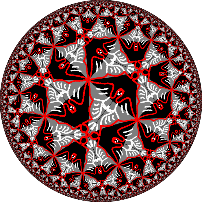
Hyperbolic tilings
In the last lecture we had a look at tilings of the hyperbolic plane. We want to tile the plane with regular $p$-gons, such that at each vertex $q$ polygons meet. Then we do a little calculation and see that for $\frac1p+\frac1q < \frac12$ there exist such tilings of the hyperbolic plane.
These tilings can be generated by a software written by Martin von Gagern from TU Munich. It is written in Java and can be downloaded from his website. I created an Escher like picture with it 🙂
Before the examns on the 21st and 26th, I will offer office hours on
Monday 18.2. 12-14 and Monday 25.2. 12-14.
Afterwards, during the semester break, there will be only office hours by appointment.
Best regards,
Emanuel
Sorry, but I didn’t find the time to blog the lectures so far but I scanned my notes. Sorry for the bad quality but I will try to improve it. But for the moment these are the available scans:
Lecture_26 Lecture_27 Lecture_28
Comment … I just printed one of the files and it looks terrible but somehow scanning pencil written notes is not as easy as I expected …
Now it’s much better – I hope 🙂
As I used various $\LaTeX$ commands and shortcuts which are not available here, I will not upload lectures 26 and 27 into the blog.
Yet they are included in the pdf version of the lecture notes which is available here.
The certificates for those who have the required amount of points in their homework are available at our secretary’s office MA 873 starting on Tue 12.02 (office hours 9:30-11:30). With the certificate you can register for the oral exam at the Prüfungsamt and sign up for a date at the secretary’s office.
Available dates so far are 21.02. and 26.02.2013. Additional dates will available before shortly before the start of the next semester.
Sorry for the delay, but I didn’t find the time earlier to add Lecture 21.
Theorem (Hyperbolic Pythagoras).
Let $\triangle ABC$ be a hyperbolic triangle with angles $\alpha$, $\beta$ and $\gamma=\frac\pi2$.
Then the lengths of the edges $a$, $b$ and $c$ satisfy
\[\cosh c=\cosh a\cdot\cosh b\,.\]
Proof.
We calculate the length in the upper half-plane model after normalizing the triangle to the following:
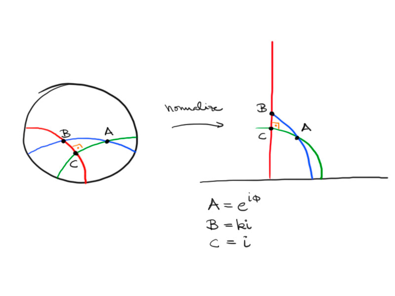
We use the formula derived for the hyperbolic distance in the upper half-plane using complex variables:
\[
\cosh d(z_1,z_2)-1
=\frac{\lvert z_1-z_2\rvert^2}{2\operatorname{Im}z_1\operatorname{Im}z_2}\,,
\]
So for the length of the edges of the triangle we obtain:
\begin{align*}
\cosh a&=1+\frac{\lvert B-C\rvert^2}{2\operatorname{Im}B\operatorname{Im}C}\\
&=1+\frac{(k-1)^2}{2k}=\frac{k^2+1}{2k}\\
\cosh c&=1+\frac{\lvert\mathrm e^{\mathrm i\phi}-k\mathrm i\rvert^2}{2k\sin\phi}\\
&=1+\frac{\left(\mathrm e^{\mathrm i\phi}-k\mathrm i\right)\left(\mathrm e^{-\mathrm i\phi}+k\mathrm i\right)}{2k\sin\phi}\\
&=1+\frac{k^2+1-2k\sin\phi}{2k\sin\phi}\\
&=\frac{k^2+1}{2k\sin\phi}\\
\cosh b&=\frac{1^2+1}{2\cdot1\cdot\sin\phi}\\
&=\frac1{\sin\phi}\,.
\end{align*}
This calculation implies the required equality.
What is the relation of hyperbolic and Euclidean triangles?
Looking at “small” hyperbolic triangles (i.e. triangles with small edge lengths and area) hyperbolic triangles behave similar to Euclidean triangles.
If the area is very small, then the sum of its interior angles is almost $\pi$.
The hyperbolic Pathagoras’ Theorem becomes the Euclidean Pythagoras’ Theorem for small edge lengths:
The Taylor series for $\cosh$ is $\cosh x=\sum\frac{f^{(k)}(0)}{k!}x^k=1+\frac12x^2+\dotsb$.
Thus $\cosh c=\cosh a\cdot\cosh b$ becomes
\[1+\frac{c^2}2+\dotsb=\left(1+\frac{a^2}2+\dotsb\right)\left(1+\frac{b^2}2+\dotsb\right)\,,\]
hence
\[1+\frac{c^2}2=1+\frac{a^2}2+\frac{b^2}2+\underbrace{\frac{a^2b^2}4+\dotsb}_{\approx0}\]
which gets $c^2=a^2+b^2$ for small $a$, $b$ and $c$.
Consider the following maps:
\[g\colon\hat\C\to\hat\C\,,\ z\mapsto\frac{az+b}{cz+d}\,,\]
where $ad-bc>0$ and $a,b,c,d\in\R$.
Here, $g$ maps $\infty$ to $\frac ac$ and $-\frac dc$ to $\infty$.
Also,
\[\tilde g\colon\hat\C\to\hat\C\,,\ z\mapsto\frac{-a\bar z+b}{-c\bar z+d}\,.\]
Theorem.
An arbitrary hyperbolic isometry of $H_+^2$ is of the form
\[z\mapsto\frac{az+b}{cz+d}\quad\text{or}\quad z\mapsto\frac{-a\bar z+b}{-c\bar z+d}\,,\]
where, again, $ad-bc>0$ and $a,b,c,d\in\R$.
Proof.
Let $\phi\colon H_+^2\to H_+^2$ be an isometry. We can construct a map $g$ which is one of the following, such that $g\circ\phi$ maps the imaginary axis onto itself and $g\circ\phi(\mathrm i)=\mathrm i$ and $g\circ\phi((0,\mathrm i))=(0,\mathrm i)$:
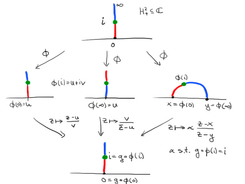
Then $g\circ\phi$ is an isometry, since $g$ and $\phi$ are. Further $g\circ\phi$ is the identity on the imaginary axis, as it is isometric and maps the imaginary axis onto itself preserving the intervals $(0,\mathrm i)$ and $(\mathrm i,\infty)$.
Now consider $x+\mathrm i y$ with $g\circ\phi(x+\mathrm i y)=u+\mathrm i v$.
We have $d(k\mathrm i,x+\mathrm i y)=d(g\circ\phi(k\mathrm i),u+\mathrm i v)=d(k\mathrm i,u+\mathrm i v)$ for all $k\in\R^+$.
Thus
\[\frac{\lvert k\mathrm i-(x+\mathrm i y)\rvert^2}{2ky}=\frac{\lvert k\mathrm i-(u+\mathrm i v)\rvert^2}{2kv}\]
and hence
\[(x^2+(k-y)^2)v=(u^2+(v-k)^2)y\]
for all $k$.
This implies $y=v$ and $u=\pm x$.
So $g\circ\phi$ is either the identity or it the reflection with respect to the imaginary axis, $z\mapsto-\bar z$.
As $\phi=g^{-1}\circ g\circ\phi$, $\phi$ is of the given type.
Lengths/distances in $H_+^2$.
Two points $P_1$ and $P_2$ in the upper half-plane model either have the same $x$ coordinate or not. If they share the $x$ coordinate the geodesic through two points is a straight line. Otherwise it is a semi-circle. Let us calculate the hyperbolic distance between two points depending on the two cases.
Case 1.
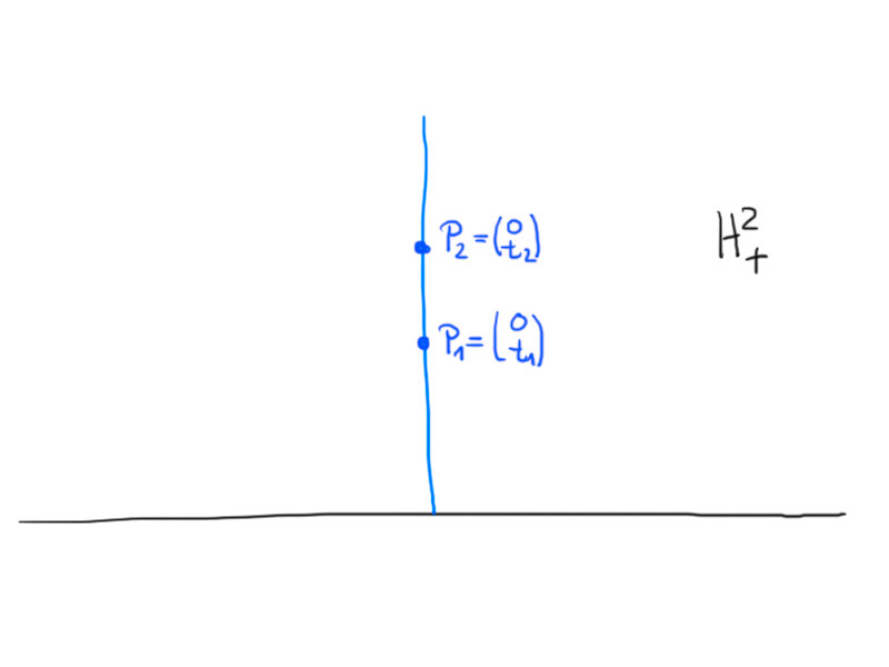
\[
\gamma\colon[t_1,t_2]\to H_+^2\,,\ \gamma(t)=\begin{pmatrix}0\\t\end{pmatrix}\,.
\]
\begin{align*}
d(p_1,p_2)&=\int_{t_1}^{t_2}\sqrt{g_{\gamma(t)}\left(\begin{pmatrix}0\\1\end{pmatrix},\begin{pmatrix}0\\1\end{pmatrix}\right)}\mathrm dt \\
&=\int_{t_1}^{t_2}\frac1t\sqrt{\left(\begin{pmatrix}0\\1\end{pmatrix},\begin{pmatrix}0\\1\end{pmatrix}\right)}\mathrm dt=\log\frac{t_2}{t_1}\,.
\end{align*}
So the length/distance only depends on the ratio $\frac{t_2}{t_1}$, not on the values.
Case 2.
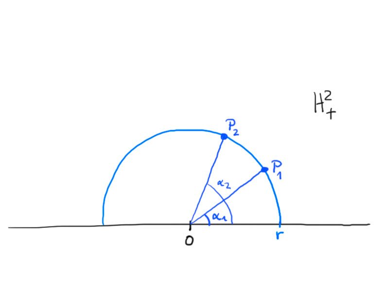
\begin{align*}
P_1&=r\begin{pmatrix}\cos\alpha_1\\\sin\alpha_1\end{pmatrix}&
P_2&=r\begin{pmatrix}\cos\alpha_2\\\sin\alpha_2\end{pmatrix}\,.
\end{align*}
Here,
\[\gamma\colon[\alpha_1,\alpha_2]\to H_+^2\,,\ \gamma(\alpha)=r\begin{pmatrix}\cos\alpha\\\sin\alpha\end{pmatrix}\,.\]
By this we get
\[d(p_1,p_2)=\int_{\alpha_2}^{\alpha_1}\frac1{\sin t}\mathrm dt=\left.\log\tan\frac t2\right\vert_{\alpha_1}^{\alpha_1}=\log\frac{\tan\frac{\alpha_1}2}{\tan\frac{\alpha_2}2}\,,\]
i.e. the distance depends on the angle, not on the radius.
Remrk.
The following maps are isometries of $H_+^2$:
Both transformations leave the Riemmanian metric invariant.
Proposition.
The distance in the Poincaré halfplane model $H_+^2\subset\C$ between two points $z_1$, $z_2$ is given by
\[\cosh d(z_1,z_2)-1=\frac{\lvert z_1-z_2\rvert^2}{2\operatorname{Im} z_1\operatorname{Im} z_2}\,.\]
Proof. Calculation using some trigonometric identities.
Let $A$, $B$, $C$ be three points in the hyperbolic plane $H^2$ not all on one line.
Then the hyperbolic triangle is given by
\[\triangle ABC=\{\lambda A+\mu B+\nu C:\lambda,\mu,\nu>0\}\cap H^2\,.\]
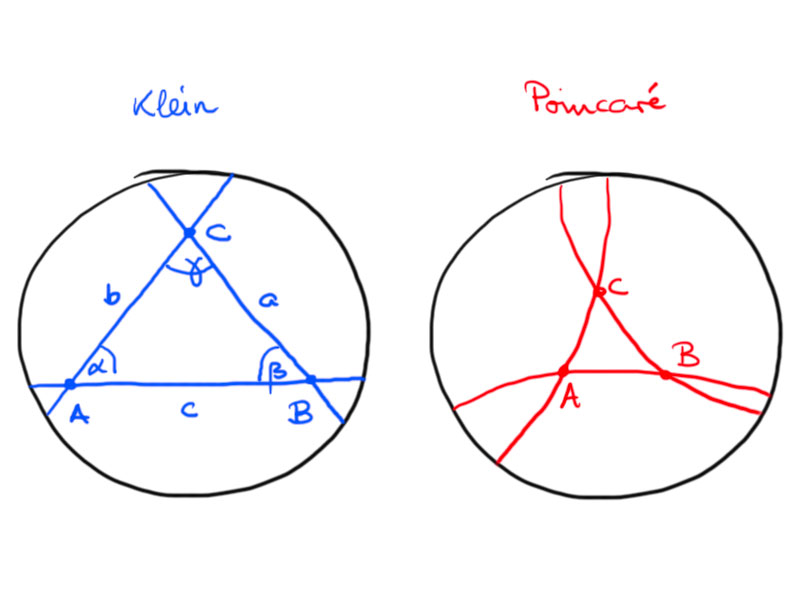
The triangle defined by $A$, $B$, $C$ in the Klein model is
\[\triangle ABC=\{\lambda A+\mu B+\nu C:\lambda,\mu,\nu\geq0,\lambda+\mu+\nu=1\}\,.\]
We label the vertices, angles and sides of a triangle as shown in the above picture.
Observation: $\alpha+\beta+\gamma<\pi$ for any hyperbolic triangle.
Consider a triangle in the Poincaré disc. We may use a hyperbolic motion to move $A$ to the center of the disc.
The angles between the hyperbolic lines at $B$ and $C$ are smaller than the angles of the Euclidean triangle, hence $\alpha+\beta+\gamma<\pi$.
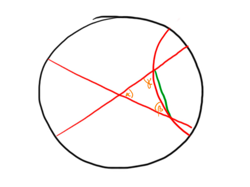
Proposition.
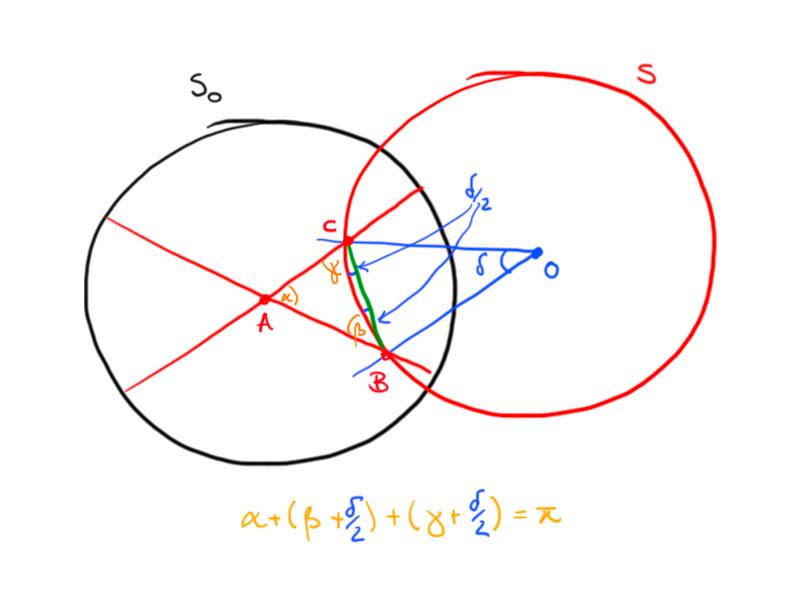
For $\alpha,\beta,\gamma>0$ with $\alpha+\beta+\gamma < \pi$ there exists a hyperbolic triangle. The triangle is unique up to hyperbolic motions.
Proof. We proof the proposition by construction: Let $\delta > 0$ such that $\alpha+\beta+\gamma+\delta = \pi$. Construct a Euclidean triangle with angles $\alpha$, $\tilde\beta = \beta+\delta/2$ and $\tilde\gamma=\gamma+\delta/2$. Then construct a circle $S$ through $B$ and $C$ such that $\angle OBC=\delta$ and $O$ on the other side of $a$ than $A$. The angles between $S$ and $b$, $c$ are $\beta$ and $\gamma$, resp. Now, construct a circle $S_0$ centered in $A$ which intersects $S$ orthogonally. Scaling this construction such that the second circle has radius $1$ yields a triangle with the prescribed angles in the Poincaré model.
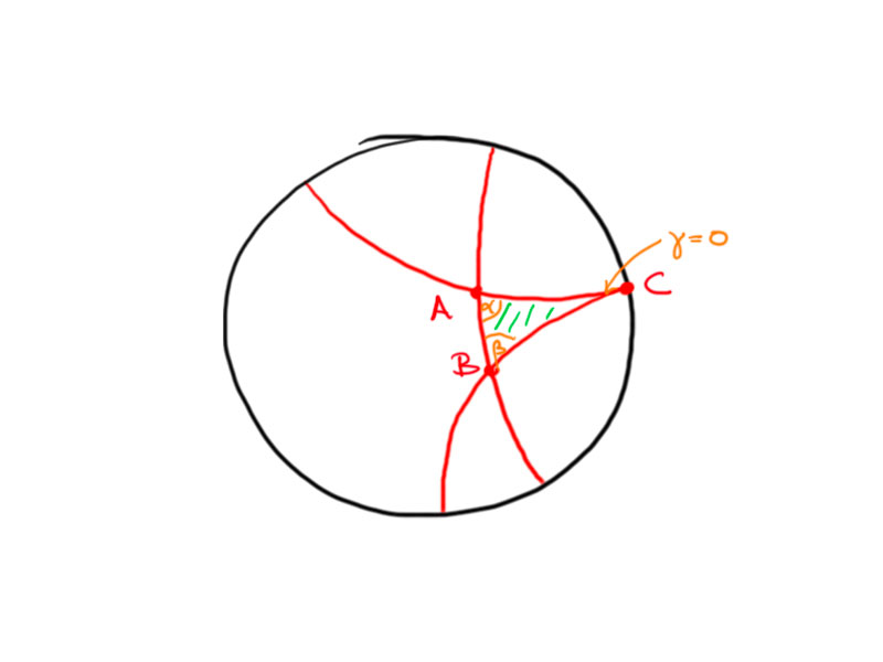
Theorem.
The area of a hyperbolic triangle with angles $\alpha$, $\beta$, $\gamma$ is $\pi-(\alpha+\beta+\gamma)$.
Proof.
Consider a triangle with one point at infinity, i.e. on the boundary of the disc in the Poincaré model.
We may normalize the picture and transform it to the upper half-plane model, such that we obtain the following picture:
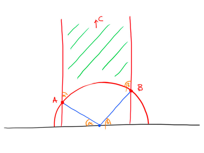
The area of the triangle is
\begin{align*}
T(\alpha,\beta,0)&=\int_{-\cos\alpha}^{\cos\beta}\int_{\sqrt{1-x^2}}^\infty\frac1{y^2}\mathrm dy\mathrm dx \\
&=\int_{-\cos\alpha}^{\cos\beta}-\left.\frac1y\right\vert_{\sqrt{1-x^2}}^\infty\mathrm dx \\
&=\int_{\cos(\pi-\alpha)}^{\cos\beta}\frac1{\sqrt{1-x^2}}\mathrm dx \\
&=\pi-(\alpha+\beta)\,.
\end{align*}
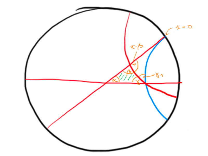
Now,
\begin{align*}
T(\alpha,\beta,\gamma)&=T(\alpha,\gamma+\gamma_1,0)-T(\gamma_1,\pi-\beta,0) \\
&=\pi-\alpha-\gamma-\gamma_1-(\pi-\gamma_1-\pi+\beta)\\
&=\pi-(\alpha+\beta+\gamma)\,.
\end{align*}