The next dates for Oral Exams in Geometry I are Friday 31.05 and 05.07.2013. You can register for the exam in the secretary’s office (Mathias Kall, MA 873).
Oral exams on 31.05. and 05.07.
Reply
The next dates for Oral Exams in Geometry I are Friday 31.05 and 05.07.2013. You can register for the exam in the secretary’s office (Mathias Kall, MA 873).
The next date for Oral Exams in Geometry I is Friday 03.05.2013. You can register for the exam
in the secretary’s office (Mathias Kall, MA 873) starting from Monday 15.04.2013.
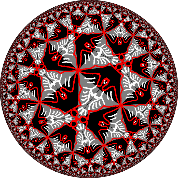
Hyperbolic tilings
In the last lecture we had a look at tilings of the hyperbolic plane. We want to tile the plane with regular $p$-gons, such that at each vertex $q$ polygons meet. Then we do a little calculation and see that for $\frac1p+\frac1q < \frac12$ there exist such tilings of the hyperbolic plane.
These tilings can be generated by a software written by Martin von Gagern from TU Munich. It is written in Java and can be downloaded from his website. I created an Escher like picture with it 🙂
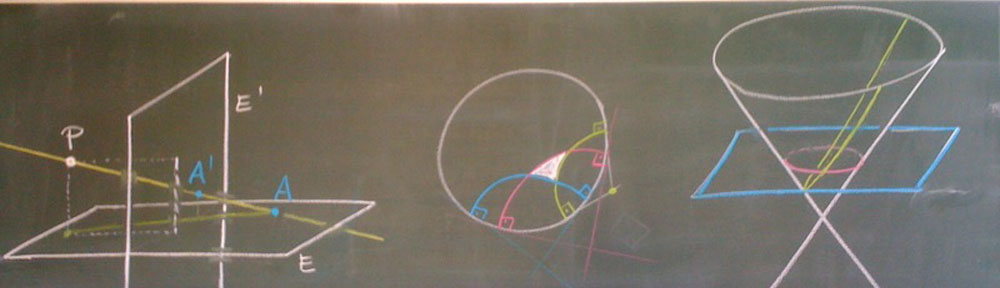
Sorry, but I didn’t find the time to blog the lectures so far but I scanned my notes. Sorry for the bad quality but I will try to improve it. But for the moment these are the available scans:
Lecture_26 Lecture_27 Lecture_28
Comment … I just printed one of the files and it looks terrible but somehow scanning pencil written notes is not as easy as I expected …
Now it’s much better – I hope 🙂
The certificates for those who have the required amount of points in their homework are available at our secretary’s office MA 873 starting on Tue 12.02 (office hours 9:30-11:30). With the certificate you can register for the oral exam at the Prüfungsamt and sign up for a date at the secretary’s office.
Available dates so far are 21.02. and 26.02.2013. Additional dates will available before shortly before the start of the next semester.
Sorry for the delay, but I didn’t find the time earlier to add Lecture 21.
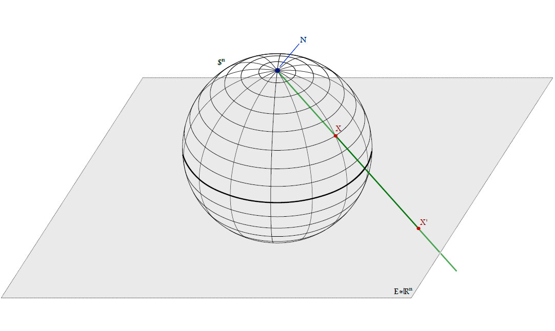
Stereographic projection
Definition. Denote the unit sphere in $\mathbb{R}^{n+1}$ by $\mathbb{S}^{n}=\left\{{x \in \mathbb{R}^{n+1}|(x,x)=1}\right\}$ and its north pole by $\mathbf{N}=e_{n+1}$.
The stereographic projection is a map $\sigma\colon \mathbb{S}^{n}\to\mathbb{R}^{n} \cup \left\{{\infty}\right\}$ from $\mathbf{N}$ to the plane
$E=\left\{{x \in \mathbb{R}^{n+1}|x_{n+1}=0}\right\} \cong \mathbb{R}^{n}$ through the equator:
\[
\sigma(X)=
\left\{
\begin{array}{ll}
\infty & \textrm{, } X = \mathbf{N}\\
l_{NX}\cap E & \textrm{, } X \neq \mathbf{N}\\
\end{array}
\right.
\]
Analytically $\sigma$ is given by
\[
\sigma(X)= \sigma\ \left(\begin{pmatrix}
x_1\\\vdots\\x_{n+1}
\end{pmatrix} \right)
= \frac{1}{1-x_{n+1}}\begin{pmatrix}
x_1\\\vdots\\x_{n+1}
\end{pmatrix}
\]
since
\[N+\lambda(X-N)=e_{n+1}+\lambda \begin{pmatrix}
x_1\\\vdots\\x_{n+1}
\end{pmatrix}
= \begin{pmatrix}
y_1\\\vdots\\y_{n}\\0
\end{pmatrix}
\Rightarrow \lambda=-\frac{1}{x_{n+1}-1}=\frac{1}{1-x_{n+1}}, X\neq N.
\]
Sphere inversion
Definition. The sphere inversion $i_{M,r}\colon \mathbb{R}^{n} \cup \left\{{\infty}\right\} \to \mathbb{R}^{n} \cup \left\{{\infty}\right\}$ in the sphere
$\mathbf{S}_{M,r}=\left\{{x \in \mathbb{R}^{n}|\left\|x-M\right\|=r}\right\}$ is given by the following conditions:
Properties of sphere inversions
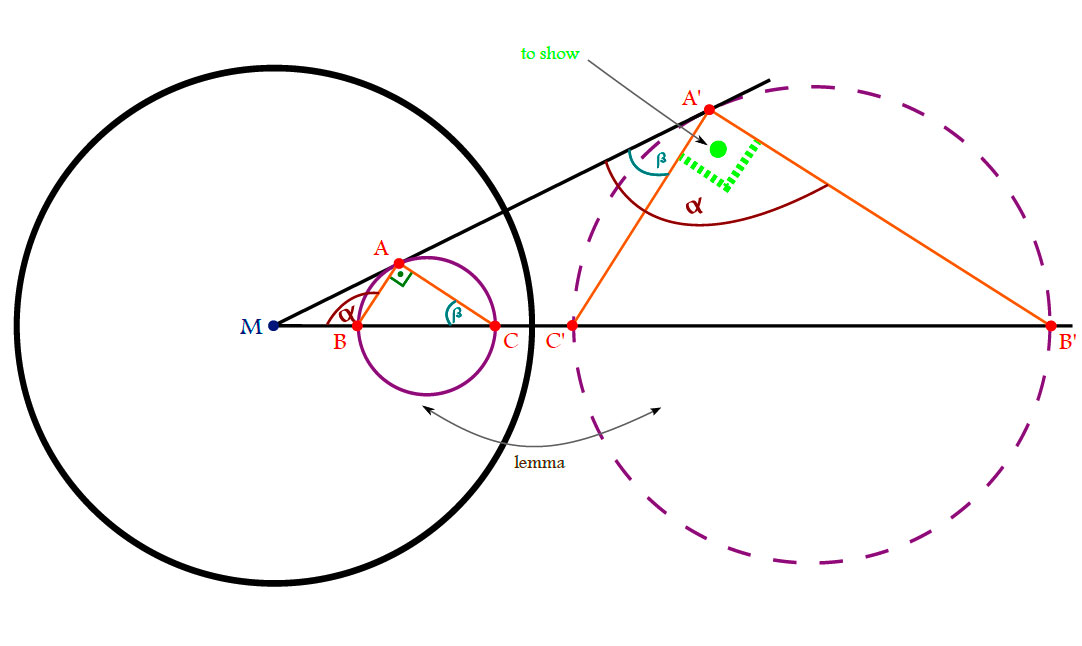
Lemma.
Proof.
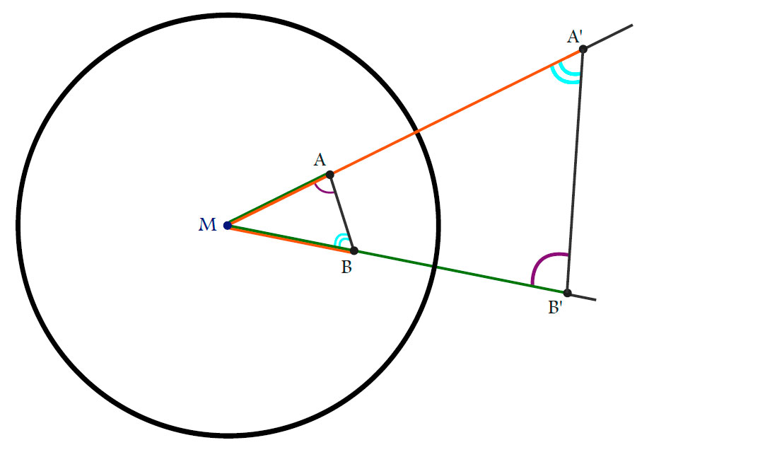
Since
\[
\left\|M-A\right\|\left\|M-A’\right\|=r^2 = \left\|M-B\right\|\left\|M-B’\right\| \iff
\frac{\left\|M-A\right\|}{\left\|M-B\right\|}=\frac{\left\|M-B’\right\|}{\left\|M-A’\right\|}
\]
we get that $\Delta AMB$ and $\Delta B’MA’$ are similar. In particular:
\[
\measuredangle MA’B’=\measuredangle ABM.
\measuredangle MAB=\measuredangle A’B’M.
\]
$\Box$
Corollary. Circles through M are mapped to lines. In particular, the line is parallel to the tangent to the circle at M.
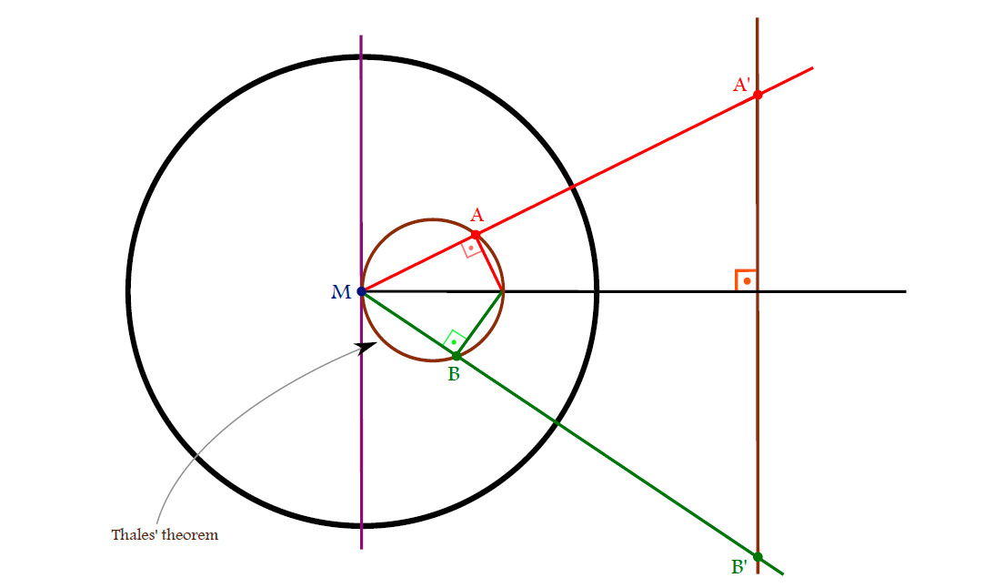
Remark. All lines are thought to contain the point $\infty$ and are considered as circles of infinte radius.
Corollary. The stereographic projection is the restriction of the sphere inversion $i_{M,r}$ with $M=e_{n+1}$ and $r=\sqrt{2}$.
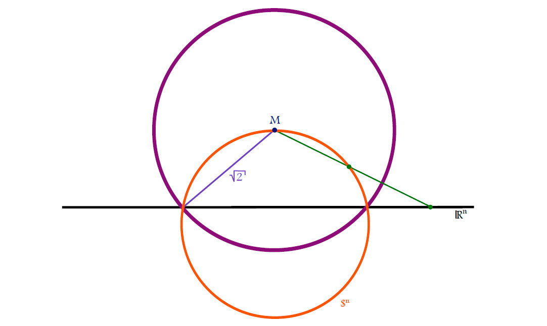
Proof.
$\Box$
Theorem. An inversion in a sphere:
Proof.
(i) Consider the following sketch:
Hence the angles $\alpha$ and $\beta$ satisfy
\[
(\pi-\alpha)+\beta+\frac{\pi}{2}=\pi \Rightarrow \alpha-\beta=\frac{\pi}{2}.
\]
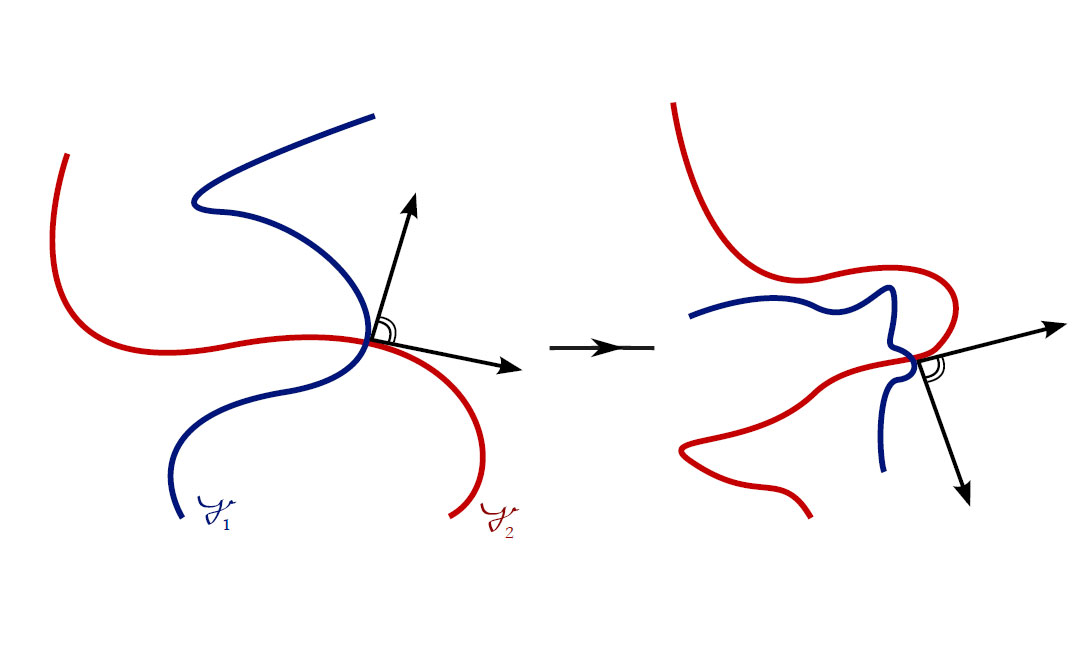
(ii) Conformality follows from the following picture
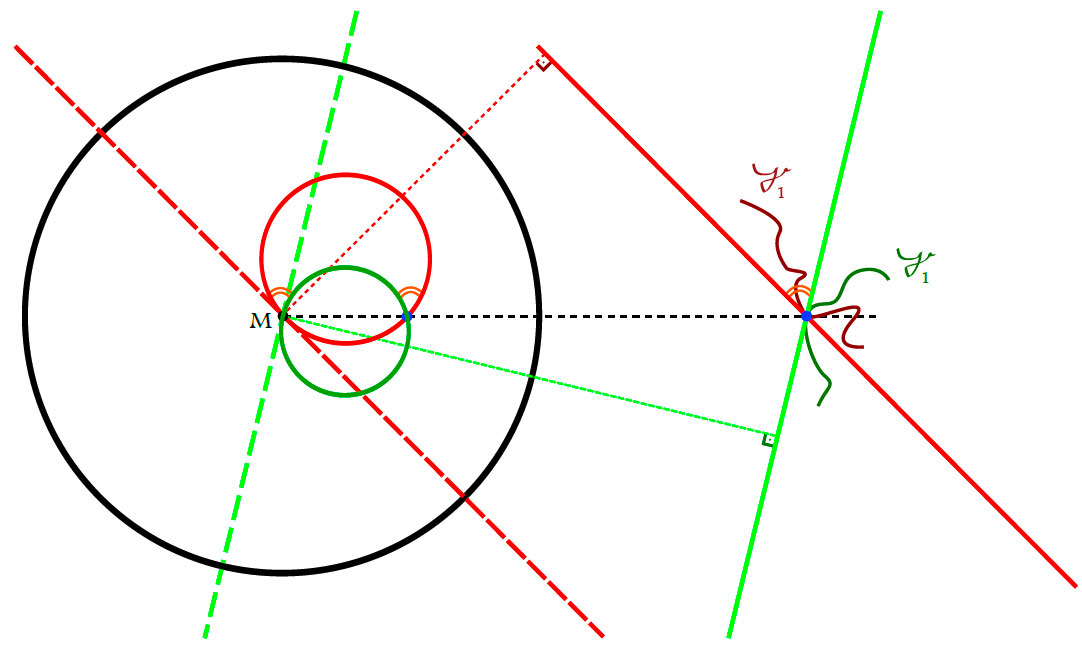
$\Box$
Remark. In general, the center of a sphere is not mapped to the center of its image by an inversion.
Corollary.
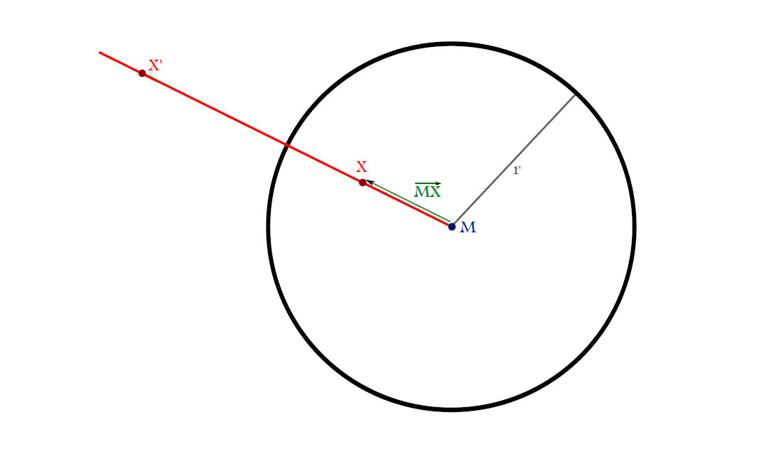
Formula for the sphere inversion.
Consider the second figure showing the general idea of a sphere inversion. Since $X’$ lies on the ray $XM$ we have $X’=M+\lambda(X-M), \lambda > 0$ and from the second requirement for the sphere inversion we obtain
\begin{align*}
&&\underbrace{\left\|X’-M\right\|}_{X’-M=\lambda(X-M)} \left\|X-M\right\|&=r^2\\
\Rightarrow&& \lambda \left\|X-M\right\| \left\|X-M\right\|&=r^2\\
\Rightarrow&& \lambda = \frac{r^2}{\left\|X-M\right\|^2}.
\end{align*}
Hence the sphere inversion is given by
\[
i_{M,r}=M+\frac{r^2}{\left\|X-M\right\|^2}(X-M).
\]
Theorem. The shortest piecewise continously differentiable curve in $H^n$ connecting two points $p$ and $q$ is the hyperbolic line segment between them. It’s length is $$d(p,q) = arcosh(-\langle p,q\rangle).$$
Let $b: V \times V \rightarrow \mathbb{F}$ be a symmetric non-degenerate bilinear form.
Definition. Let $U \leq V$ be a vector subspace. Then
\[
U^{\perp} = \{ v \in V \: | \: b(u,v) = 0, \: \forall u \in U \}.
\]
If $U = \{u_1,…,u_k\}$ then
\[
U^{\perp} = ( \text{span} \; U )^{\perp} = \{ v \in V \: | \: b(u_i,v) = 0, \: \forall i = 1,…,k \}.
\]
We call $U^{\perp}$ the orthogonal complement of $U$.
Remark. dim $U^{\perp} =$ dim $U^0 = n – k$, if dim $U = k$ and dim $V = n$.