Hi! In this tutorial, we will learn the fundamentals of volumes and also get started with python coding! That is an incredible amount of fun!
Volumes
The most intuitive 3D mesh to fill up space is to dissect space into many little cubes. Such a box of dissected cells can be placed using the volume node.


Each cell can now carry an attribute. Normal meshes fill up surfaces only but 3D mesh fills up volume.
Volumes and Velocity
One can initialize this volume to carry vectors that we call velocity in our case.
The thing is, volumes are a bit special (like all of us). They are not points, vertices, primitives. They are their own special kind and get their own volume wrangle node for manipulations. Inside the volume wrangle, you can then access attributes such as v@P for the cell position and v@velocity for the vector we just defined. This means that you can use v@P as your input to a function to evaluate a velocity field.
Here is an example of a spinning vector field. We then use a few nodes to sample points inside the volume and then trail out the velocity field using these points as starters. Learn to use the volume trail node for volume inspection.


We can also animate motion in the velocity field using solver nodes! For that, we must first convert the volume into the OpenVDB volume format. The sampled points from above are then added to the solver and advected using the VDB advect points node. Straight forward. VDB is also cool because it lets us compute gradients and curls easily using the VDB analysis node.


Volume and Scalar Functions
The velocity vector above was actually just 3 scalar functions. Kind of like three kids stacked up and wearing a big trench coat to appear like an adult. If we, however, stick to just scalar functions we can build surfaces with that!
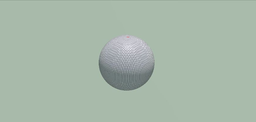
For example, we create a scalar f@f and assign the function f@f = $1-4r^2$; to it where r is the distance to the origin. We can then create isosurfaces by meshing the level set to a given value of f@f using the convert volume node. For example, tracing out the values of f@f = 0.5 will give us a small sphere of radius $\frac{1}{\sqrt{2}}$. However, choosing negative values will give us something that looks like the cut out of a sphere from a box.

Volumes Being Useful
Each volume cell (Voxel!) has its address as i@ix, i@iy, i@iz. You can read useful calls here. What is important is that even though you only have 10x10x10 voxels like in this example, you can sample interpolated values in between these voxels. For example attribute from volume node lets you do this. This can also be done in code:
float volumesample(<geometry>geometry, string volumename, vector pos)
Volumes from Surfaces
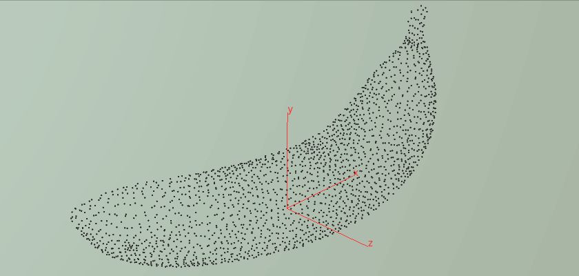
We just saw how to create a surface from a volume, but we can also create a volume using a surface using the VDB from polygon node. Given for example a banana mesh with a tangent vector field on it, we can build a volume around the mesh and advect points on the surface. The node sequence below shows you how to do this. This is fantastic for visualizing vector fields. Volumes can also be generated to get a signed distance field for your mesh.

Python and Houdini
Python is strong because it comes with many great operators that we would like to use. SciPy, for example, comes with sparse matrix builders and solvers that we absolutely need for exterior calculus applications.
Head to the download section and get the hip files of this Tutorial 04. There, python is used with careful documentation. In this lesson, we will not make use of SciPy yet.
Instead, you will learn how to read attributes in Python and save attributes and matrices for later access.

Installing SciPy for Next Tutorial
We will need SciPy soon and for that I wish you to install it. Things work differently for Windows, Mac, and Linux so I can’t just give a simple answer on how to do so. Sadly, the newer versions of Houdini really mess up when it comes to custom python packages. You can try to use it with your version but if Houdini fails to find the SciPy package then try it using an older version.
Here is an old tutorial that worked well with Houdini 16.5 and below. (be sure to read it carefully)
I have noticed that I could not check out a free license for 16.5 after installing it now. However, I managed to install the newest version, then check out the license, and then I was able to continue using Houdini 16.5 as usual (both versions can coexist on your machine). Perhaps try that before following the tutorial above if all else fails.
Here you find the previous version of Houdini:
https://www.sidefx.com/login/?next=/download/daily-builds/
You will know that SciPy works as soon as the import SciPy command does not fail.
