Tutorial 08: Life with Boundaries

Today we will learn about the inclusion of boundaries in your DEC setup. This will be an essential lesson in solving Poisson problems $\Delta u = f$.

This tutorial comes with implementation files in the download section.

Boundaries

Boundaries force us to adapt which then opens up the door for new ideas. This also applies to discrete exterior calculus (DEC). In this course, we have often avoided boundaries due to the added complications that we get through them but today we will shed some light on this topic which will allow us to create waves and heat simulations that realistically deal with boundaries.

DEC life with Boundaries

So how should our DEC build deal with boundaries? The answer is surprisingly simple. The exterior derivatives $d$ does not change at all while the Hodge-star operators $\star$ only have to adjust their values at the boundaries a bit.

Always keep this image in your mind:

What happens to $\star_k$?

Let $\sigma_k$ be the k-measure used for the Hodge-star computation. In our euclidean settings this means that:

• $\sigma_0$ counts points
• $\sigma_1$ measures length
• $\sigma_2$ measures area
• $\sigma_3$ measures volume

The discrete Hodge-star $\star_k$ is then defined as a diagonal matrix with the ratio between the dual measure and the primal measure.

$$ (\star_k)_{ii}(e) = \frac{\sigma_{n-k}(\text{dual}(e))}{\sigma_k(e)}$$

Where $e$ is a either a point, edge or face.

For our 2D surface case you can now look at the above image and see the following:

• The primal graph measures are not influenced by the boundary.
  • The number of points is fixed.
  • The edges lengths stay the same.
  • The face areas stay the same.
• The dual graph, however, does affect the measures at the boundary!
  • Dual point areas at the boundary are now smaller than before.
  • Dual edges are also cut shorter.
  • Dual faces are not affected as they are measured by counting.

Implementations of $\star$ with boundaries now only have to compute slightly different measures at the boundaries. That’s it!

What happens to $d$?

Nothing! That is actually crazy.

• $d_0$ is just a derivative along edges in the primal graph. This operator does not even notice the presence of a boundary.
• $d_1$ is a derivative between faces in the primal graph. A boundary edge is not between faces. There is nothing to adjust for at the boundary.
• $d^*_0$ is the dual derivative between dual points (primal face centers). Just like in $d_1$, there is no face beyond the boundary and thus no derivative there.
• $d^*_1$ is the dual derivative between dual faces (primal points). Just like with $d_0$, nothing changes as the derivative along the primal edges are well defined even at the boundary.

For the 2D surface case we still have the computationally super convenient formula

$$d^*_1 = d_0^{\intercal}$$

$$d^*_0 = d_1^{\intercal}$$

And the boundary respecting Laplacian still obeys the old formula as usual

$$\Delta = \star d \star d + d \star d \star$$

In fact, the DEC build assets you received earlier already do this.

Living with Conditions

Ok cool. We have now a DEC setup with a Laplacian but how do we actually solve the heat equation or the wave equation with this?

Solving a differential equation on a domain $M$ with a boundary will require boundary conditions, possibly multiple distinct conditions for different parts of the boundary. The choice of this boundary condition strongly depends on the context. This page has a nice list of possible conditions. The main conditions that show up again and again in graphics are the following:

• Dirichlet boundary condition:
  • Solving for $f$ with prescribed values of $g_D$ at the boundary $\partial M_D$
  • How to remember: “Dirichlet” is “dictating” the exact values.
  • Example: solve $\Delta f = 0$, given $f|_{\partial M_D}=g_D$.
    • Meaning: Solve for the steady-state heat distribution with prescribed heat in certain areas. Solving for a harmonic function.

• Neuman boundary condition:
  • Solving for $f$ with prescribed flux $g$ at the boundary $\partial M_N$
  • How to remember: “Neuman” is dealing with the “normals”.
  • Example: Solve $\Delta f = \partial_t f$, given $\frac{\partial f}{\partial n}|_{\partial M_N} = g$.
    • Meaning: Solve for heat flow with prescribed incoming and outgoing heat sources.
  • Example: Solve $\Delta f = \partial^2_t f$, given $\frac{\partial f}{\partial n}|_{\partial M_N} = 0$.
    • Meaning: Wave equation with walls that prevent the wave from leaving.

Solving with Conditions

How do I implement these conditions into my favorite DEC setup? We will stick to the geometric interpretation of the heat flow to describe what happens.

Dirichlet Condition

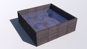
Ok, simple example. Let’s say you want to solve $\Delta f = 0$ with prescribed $f|_D = g_D$. Example: you have some square shape with blue and red marked areas where constant heating/cooling is applied. We want to compute the steady-state heat distribution that the heat equation converges to.

In this case the Dirichlet boundary condition is set on points and we are trying to solve the heat $f$ as a 0-form.

The way to approach this is through matrix slicing. We already know that some points are going to be fixed. In our case we will call these points boundary points. Let B be the set of boundary points and I the set of interior points. All the DEC operators can be permuted since their order only dependent on the enumeration of the points, edges and faces. These enumerations are arbitrary. Imagine now that we would re-enumerate all our points in such a way that we first count all the interiour points I and then count all the boundary points B. Then our equation would look like this:

$$\Delta f = \begin{bmatrix}
\Delta_{II} & \Delta_{BI}\\
\Delta_{IB} & \Delta_{BB}
\end{bmatrix} \begin{bmatrix}
f_I\\
f_B
\end{bmatrix} = 0$$

Where the I and B mark what parts of the matrix act on the interior and boundary points respectively. Since $f_B$ is already directed by the Dirichlet condition we only want to solve for $f_I$. This is actually quite straight forward. Just solve the following sliced equation for $f_I$:

$$\Delta_{II} f_I = -\Delta_{BI}f_B$$.

Then stich $f_I$ and $f_B$ together on $M$ and that’s it! Solving this equation for the above example then gives us this heat distribution:

This is what this solver would give us if we had only specified half of the top and bottom boundary to have a fixed temperature value:

Here is an example of a spiral where only the tips are heated or cooled respectively:

And here a strange slice of cheese where certain corners got marked with the Dirichlet condition:

Note!: Solving this type of problem with prescribed values will happen again and again, and as you might have noticed, we have not used the fact that our boundary points are actually on the boundary. You could use this to fix values on the inside of the set too. However, the good thing about having these conditions on boundaries is that you are guaranteed a solution as long as your set $M$ is compact and connected. If your Dirichlet conditions draws a closed curve inside your set then you are effectively splitting the set and solving multiple Dirichlet problems at once.

In the examples above we marked some boundaries with conditions, but not all of them! What happened there? Next, we will show that not specifying anything at the boundary is equivalent to setting a zero Neumann boundary condition.

Neuman Condition

Let’s solve for the steady-state of the heat equation again but this time without any prescribed temperatures. Instead, we will fix the amount of heat traveling in to and out of the surface. For example, we take a grid and watch how the heat enters from the sides.

The heat flow corresponding to this steady-state that we are looking for looks like this:

$$ \partial_t u_t= \Delta u_t + \star d g $$

where $g$ is a flux 1-form along the dual-edge (normal to the boundary) specifying the flux with the boundary. $g=0$ on the interior.

Since we work with temperatures on points only we can go ahead and replace $\star d g$ by $\tilde{g}$ specifying the incoming/outcoming temperature at that point.

$$ \partial_t u_t= \Delta u_t + \tilde{g} $$

This time we don’t have to slice any matrices. The Neuman steady-state equation is the following:

$$ \star d \star d f = -\tilde{g} $$

This is just a Poisson problem. We move the $\star$ to the other side for computational convenience and then solve for $f$. This is what it looks like for the test case constructed above:

But wait! When can we assume this equation to have a solution? The answer is geometrically simple: When the mean boundary flux is 0. Why? because if you continuously pump heat in and out of a system, stability can only occur if the amount of heat coming in and the amount of heat going out is the same. If this is not the case, the system will have infinite heat or negative infinite heat as the heat flow continues. This condition also guarantees that the divergence theorem holds:

$$ 0 = \int_M \Delta f = \int_M \nabla \cdot \nabla f = \int_{\partial M} n \cdot \nabla f = \int_{\partial M} \frac{\partial f}{\partial u } $$

Here is another example of flux entering and leaving a system.

Notes!: This result is really cool because it means that if $g=0$ on the boundary (no flux leaving the system) we have to implement exactly nothing! This is actually how we got away in the Dirichlet solutions above without specifying Dirichlet conditions on all the boundary points.

Solving for Dirichlet and Neuman condition at the same time!

This is simple. Just set up the Neuman problem and start slicing. Let us solve $\Delta f = -g$ by looking at

$$L f = -\star g$$

($L = d\star d$) Let us split the boundary $\partial M$ into a Dirichlet part $\partial M_D$ and a Neuman part $\partial M_N$ (these two sets do not intersect).

$$\partial M = \partial M_D \cup \partial M_N$$

First, we slice our matrix as above for the Dirichlet boundary. We define $I_D:=M – \partial M_D$ as the interior points with respect to the Dirichlet boundary and $B_D$ as the Dirichlet boundary itself. This will give us this sliced version of our equations:

$$ L_{II_D} f_{I_D} = -L_{IB_D}f_{I_B} – \star_{II_D} g_I$$

Then we just solve this.

How to Implement this in SciPy

This is where matrix slicing gets its name from. We are solving for $\Delta f = -g$ with Dirichlet and Neuman conditions. This is equivalent to solving $L f = -\star g$ with $L = d \star d$. Let $\text{bdy_d}\in \mathbb{Z}^n$ be a vector such that

$$\text{bdy_d}_i=\left\{ \begin{array}{ll} 1 \in \partial M_D \\0, \text{else} \end{array} \right\}$$

Let $\text{bdy_d_val}$ and $\text{bdy_n_val}$ be the vectors containing the Dirichlet and Neuman boundary data respectively. Then we can get $L_{II}$ and $L_{IB}$ by eliminating rows and colums that are unwanted. We create two complementary numpy vectors

and use them for sclicing

The same slicing has to be done for star0. The right hand side (rhs) also has to be sliced correctly with the Dirichlet and Neuman boundary data.

We can then solve

and then combine this solution with the Dirichlet boundary data

Heat Flow Example

Let’s solve $\partial_t f = \Delta f + g$ with Dirichlet and Neuman boundary conditions. Previously we solved this equation without (g=0) boundaries using

$$(\star – hL)f_{k+1} = \star f_k$$

Now this derivation can also be performed using slicing like this:

$$(\star_{II} – hL_{II})f_{I,k+1} = \star f_{I,k} – h(L_{IB}f_D + \star_{II} g_I)$$

For example:

Wave Equation Example

For waves, a Dirichlet condition does not really make sense. The most reasonable boundary condition is to prevent the wave from leaving the domain. This corresponds to a zero Neuman condition. As we have learned above having $g=0$ means that we have to change absolutely nothing! As long as your DEC build has the right dual edge weights and point weights everything works fine out of the box. We still solve

$$f_{t+h} = h^2\Delta f_t + 2f_t – f_{t-h}$$

and get valid reflections at the boundary.

More Notes

• • If in doubt, check the residual of what you just solved. So if your solver just returned your $x$ that allegedly solves $\Delta x = f$ then compute the residual.
    $$ r:= \Delta x – f $$
    If this isn’t tiny small then something went wrong. This is a nice check when you have to deal with harmonic generators.
  • Check out the talk from Solomon/Crane/Vouga Laplace-Beltrami: The Swiss Army Knife of Geometry Processing (2014).
  • A more natural boundary condition for the heat equation would be a Robin-boundary condition. With it, the flux at the boundary is dependant on the value at the boundary. This is accurate for the cool down process where the outside has a constant temperature (e.g. the outside wheater) and the inside cools or heats up depending on the temperature difference.