In today’s tutorial, we will mathematically prove that we will all die and be forgotten and then simulate this. We will then play with waves.
Please check out the download folder and check out the .hip file of this tutorial. It will contain a functional DEC build with a heat flow example. I have noticed that many of you used for loops to build the sparse matrix. The file shows that this is not necessary.
Entropy
Given a 0-form $u_t:M\rightarrow \mathbb{R}$ that represents temperature at time $t$ on our surface $M$, the dynamics of the heat is given by the heat equation:
$$\partial_t u_t = \Delta u_t = \star_0^{-1} d_1^*\star_1 d_0 u_t$$
we can define entropy to just be the n-form
$$\sigma_t:=\star_0 \log u_t$$
The interpretation of this function does not matter at all for the math and its implications that follow from it. We can define the total entropy as
$$ S(t):= \int_M \sigma_t$$
The Amazing Thing about Entropy
In a closed system ($\partial M = \emptyset$), the total entropy’s derivative is always positive, which is also often referred to as the second law of thermodynamics.
$$\frac{d}{dt}S(t) \geq 0$$
We show this now:
$$ \frac{d}{dt}S(t) = \int_M \partial_t \sigma_t = \int_M \star_0 \partial_t \ln u_t$$
$$
= \int_M \star_0 \frac{1}{u_t}\partial_t u_t
= \int_M \star_0 \frac{1}{u_t} \Delta u_t $$
$$
= \int_M \star_0 \frac{1}{u_t} \star_0^{-1} d_1^*\star_1 d_0 u_t
= \int_M \frac{1}{u_t} d_1^*\star_1 d_0 u_t$$
$$
= \int_M d_1^*\left( \frac{1}{u_t} \star_1 d_0 u_t \right ) – d_0\left( \frac{1}{u_t}\right)\wedge \star_1 d_0 u_t$$
$$
= \int_M d_0\left( -\frac{1}{u_t}\right)\wedge \star_1 d_0 u_t
= \int_M \frac{1}{u_t^2} d_0u_t \wedge \star_1 d_0 u_t $$
$$
= \int_M \star_1\frac{1}{u_t^2} |d_0u_t|^2 dp \geq 0$$
Here we used integration by parts together with stokes theorem.
The Implications
So! Why should we care? Well actually we don’t have to, but if we assume that our universe $M$ is an isolated system with finite energy and we believe the laws of thermodynamics to be true, then the following is true in our universe:
The fact that $S$ can only increase in time shows us that the system has no loops. This is a profound statement to make about $u$ on $M$. Think of it this way: no matter how the dynamics turn out, the state as it was before can never ever return at a later time because this would imply that the total entropy would reach the same value again.
When does $\frac{d}{dt}S(t) = 0$? From the equations in our derivation above, we see that this is indeed the case when $d_0u_t = 0$. In that case, $M$ is at thermal equilibrium, meaning that no heat difference exists anymore.
At the thermal equilibrium, everything will come to an end. All energy available for mechanics will have dissipated into heat and no more life will be able to exist. This is called the heat death of the universe.
The Discrete Version
The discrete version can also be computed in Houdini.
$$ S(t):= \sum_i \sigma(p_i,t) = \sum_i \text{f@point_weight*log(f@u)}$$
For the heat flow on the bunny, you will see this term rise all the time. However, if you initialize your $u$ with many 0 values then log(0) will cause problems. You can get around this by adding a mini-mini-mini amount of heat everywhere. This is ok because true 0° Kelvin temperature can never be reached.
If our universe was bunny-surface shaped, then the heat flow together with this computation would be a valid simulation of entropy.
Splish Splash Waves
Let $u_t:M\rightarrow \mathbb{R}$ be a 0-form. The wave equation is given by
$$\partial_t^2u_t = \Delta u_t$$
We have not yet given $u$ a specific physical meaning. This is because many things in life obey the wave equation in different contexts. For this class’s sake, we can simply assume that this is the hight of the water on a surface $M$.
We have our DEC build ready, the only thing left to do is to find a suitable discretization of this equation to simulate it.
The simplest approach will actually be a really good one (Verlet integration). We use a simple discretisation of the second derivative:
$$\partial_t^2 u_t = \frac{1}{h}\left( \frac{u_{t+h} – u_{t}}{h} – \frac{u_{t} – u_{t-h}}{h} \right)$$
$$ = \frac{u_{t+h} -2 u_{t} +u_{t-h} }{h^2}$$
Set this equal to $\Delta u_t$ and solve for $u_{t+h}$:
$$u_{t+h} = h^2\Delta u_t + 2u_t – u_{t-h}$$
That’s it! Since this is a second order differential equation we need to track $u_t$ and $u_{t-h}$. This is simple in our case because we just have to store the value of $u_t$ from the previous time step.
Also, keep in mind that for the initial values for these simulations it is not enough to just define $u_t$, you have to define $u_{t-h}$ somehow too.
You will have fun with this in your homework.
Painting in Houdini. Painting attributes.
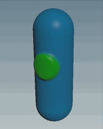
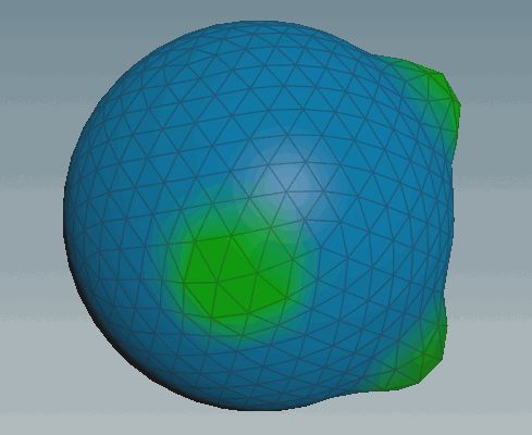
To design your initial condition for $u$ on the surface we can abuse the paint tool. First we initialize every $f@u = 0.5$ on all points. Then simply place a paint node and select the white color (value 1) and check “overwrite color” and set it “u”. Then with the paint node selected, however over the scene view and hit enter to activate paint mode and start painting. Press escape to finish paint mode. Repeat this with a black paint node (value 0). Then use a point node to map these values form -1 to +1.

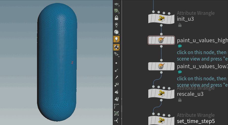
In this case, later down the nodes we use the “u” attribute to recolor and displace the surface. This is why the painting of the attribute “u” is visible.
the final visualization looks like this.