Historical Remarks
The word geometry is of Greek origin ($\gamma\varepsilon\omega\mu\varepsilon\tau\rho\iota\alpha$) and means “measurement of the earth”. But the first accounts were found in Egypt and Mesopotamia (today Iraq) around 2000 BC. It was known how to calculate simple areas and volumes and people of that time already had an approximation of $\pi$. But no general statements/theorems and proofs were found. Around 600 BC in Greece, Thales was the first to deduce theorems from a set of axioms. At about 300 BC, Euclid wrote the book Elements in which he states the five axioms of what is today called Euclidean geometry. His fifth axioms is known as the parallel postulate and can be phrased as follows:
Given a line and a point not on this line, there is a unique line through the point parallel to the line.
In the following centuries people tried to prove this postulate from the other four but were not successful. As we know today, there exist other geometries that violate this postulate. These geometries are called Non-Euclidean Geometries: e.g. spherical geometry, hyperbolic geometry (developed independently by Lobachevsky and Bolyai; 19th century), projective geometry (Poncelet; 19th century). Another important development was the introduction of coordinates in the 17th century by Descartes and Fermat. The geometry starting from axioms is called synthetic geometry and the geometry based of coordinates analytic geometry.
Course Content
In this course we will consider projective, hyperbolic and Moebius geometry. And if time permits we might also have a look at Lie, Laguerre, or Pluecker geometry. The aim is to provide you with lots of geometric images and their analytic counterparts.
The continuation of this course is a speciality of the TU Berlin and is called Geometry II: Discrete Differential Geomtry. It is concerned with intelligent discretizations of smooth theories, e.g. from differential geometry and dynamical systems. The recently established SFB/TR Discretization in Geometry and Dynamics will enlarge the opportunities to do further research in this direction.
Perspective example
We start with an example painters have to deal with when capturing a scene in a painting, cf. “Albrecht Dürer: Mann beim Zeichnen einer Laute, 1525”.
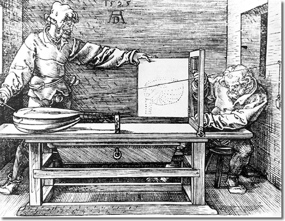
Albrecht Dürer: Mann beim Zeichnen einer Laute, 1525
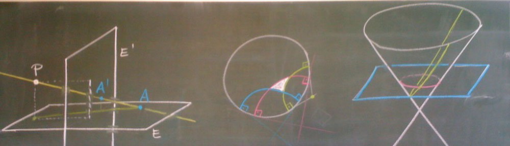
We will consider the projection of a spatial scene onto a plane but the central projection of one plane onto another. So consider two planes $E,E’ \subset \R^3$ that are not parallel and a point $P \in \R^3$ that does not lie on the planes as shown in the following picture.
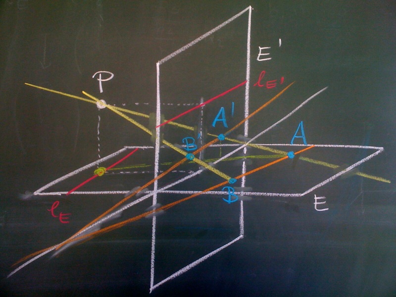
Figure 1: Central projection of the plane E to the plane E’ through the point P.
The projection $\pi : E \to E’$ does the following: let $A$ be a point on the plane $E$. Then
\[ A’ = \pi(A) = \mathrm{line}(P,A) \cap E’ \]
Problem: We would like to have a bijective projection map, but the points on the line $\ell_E$ are not projected to any point on $E’$, since the plane spanned by $\ell_E$ and $P$ is parallel to $E’$. Further the points on $\ell_{E’}$ lack a preimage, since the plane spanned by $\ell_{E’}$ and $P$ is parallel to $E$. The lines $\ell_E$ resp. $\ell_{E’}$ are the vanishing lines of $E$ resp. $E’$.
Idea: Introduce two additional lines $\ell_{\infty}$ and $\ell_{\infty}’$ to $E$ and $E’$, respectively. The points on $\ell_E$ will be mapped to $\ell_{\infty}’$ and the points on $\ell_\infty$ are mapped to the points on $\ell_{E’}$. The lines $\ell_{\infty}$ and $\ell_{\infty’}$ are called the lines at infinity.
Done in the right way, this yields a bijective projection $\pi : E \cup \ell_{\infty} \to E’ \cup \ell_{\infty’}$. Parallel lines in $E$ are mapped to concurrent lines in $E’$. The intersection point $Q’$ of the images of parallel lines lies on the vanishing line $\ell_{E’}$. The point $Q’$ is the image of the “intersection point at infinity” $Q \in \ell_{\infty}$ of the original parallel lines.
Example. We are now able to construct a perspective drawing of a chessboard given the image of the first square. The chessboard contains two families of obvious parallel lines, namely the horizontal and vertical directions. But the diagonals of the chessboard are also parallel. Hence we obtain four points on the vanishing line on $E’$, one for each parallel family. These allow us to construct the perspective projection.
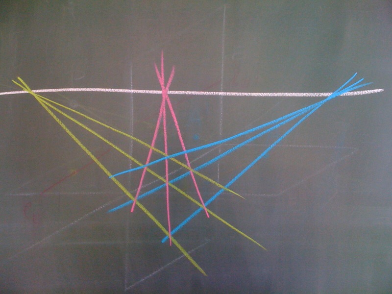
Construction of a perspective image of a chessboard.
Question. Can you construct the perspective image of the first square given the position of the chessboard, your position (the “eye” point), and the position of the plane projected onto?
Now let us turn to the analytic treatment of the above example. Let the two planes and the point be the following:
\begin{align*}
E &=
\left\{ \begin{pmatrix}x_1\\x_2\\x_3\end{pmatrix} \in \R^3 \,|\, x_3=0 \right\}, \\
E’ &=
\left\{ \begin{pmatrix}x_1\\x_2\\x_3\end{pmatrix} \in \R^3 \,|\, x_1=0 \right\} \text{, and} \\
P &= \begin{pmatrix}-1\\ 0\\1 \end{pmatrix}.
\end{align*}
As the planes are two dimensional subspaces we assign two coordinates to each of the points on either of the planes, i.e. $A = \tbinom{a_1}{a_2}$ and $A’ = \tbinom{a_1′}{a_2′}$. We calculate the coordinates of $A’$ from $A$ by considering the line through $A$ and $P$ and its intersection point with $E’$. Thus we need to solve:
\begin{align*}
&\begin{pmatrix} a_1\\a_2\\ 0 \end{pmatrix} +
\lambda (\rvector{-1\\ 0\\1} – \rvector{a_1\\a_2\\ 0}) = \rvector{0\\a_1’\\a_2′} \\
\Rightarrow\quad&
a_1 + \lambda(-1-a_1) = 0 \quad \Rightarrow
\lambda = \frac{a_1}{1+a_1}.
\end{align*}
Hence we obtain
\begin{align}
a_1′ &= a_2 + \frac{a_1}{ 1+a_1}(-a_2) = \frac{a_2}{1+a_1} \\
a_2′ &= 0 + \frac{a_1}{1+a_1}(1-0) = \frac{a_1}{1+a_1} \quad \text{and thus} \\
A’ &= \pi(A) = \frac{1}{1+a_1} \rvector{ a_2\\a_1}.
\label{eqfract}
\end{align}
Whenever there is a fractional linear transformation it is worth to introduce homogeneous coordinates to linearize the equations, i.e. introduce $\svector{b_1\\b_2\\b_3}$ with $b_3 \neq 0$ for $\svector{a_1\\a_2}$ (unique up to non-zero scaling) with $a_1 = \tfrac{b_1}{b_3}$ and $a_2 = \tfrac{b_2}{b_3}$. Similarly, $\svector{b_1’\\b_2’\\b_3′}$ with $b_3′ \neq 0$ for $\svector{a_1’\\a_2′}$ with $a_1′ = \tfrac{b_1′}{b_3′}$ and $a_2′ = \frac{b_2′}{b_3′}$. If we then look back at Equation \ref{eqfract} we obtain the following relation between the homogeneous coordinates:
\begin{align*}
&\frac{b_1′}{b_3′} = a_1′ = \frac{a_2}{1+a_1} = \frac{b_2/b_3}{1+b_1/b_3} =
\frac{b_2}{b_1+b_3}
\quad \text{and}\\
&\frac{b_2′}{b_3′} = a_2′ = \frac{a_1}{1+a_1} = \frac{b_1/b_3}{1+b_1/b_3} =
\frac{b_1}{b_1+b_3} \\
\Rightarrow \quad&
b_1′ = b_2,\;
b_2′ = b_1,\;
b_3′ = b_1 + b_3.
\end{align*}
Hence in homogeneous coordinates the projection has become a linear(!) map:
\[
\rvector{b_1\\b_2\\b_3} \; \mapsto \rvector{b_1’\\b_2’\\b_3′} =
\begin{pmatrix}
0&1&0\\
1&0&0\\
1&0&1
\end{pmatrix}
\rvector{b_1\\b_2\\b_3}.
\]
But what happens to the vanishing line $\ell_E$? The points on the vanishing line have coordinates $\svector{-1\\a_2}$. Introducing homogeneous coordinates this amounts to $\svector{b_1\\b_2\\b_3}$ with $b_3 \neq 0$ and $\tfrac{b_1}{b_3} = -1$. Thus $b_1 + b_3 = 0$ and in particular $b_1 \neq 0$. For the image of such a point under the projection these conditions imply:
\[
\begin{pmatrix}
0&1&0\\1&0&0\\1&0&1
\end{pmatrix}
\rvector{b_1\\b_2\\b_3} = \rvector{b_2\\b_1\\b_1+b_3} = \rvector{b_2\\b_1\\ 0}.
\]
The image point does not correspond to a point on the plane, because the last coordinate is zero contradicting the assumption $b_3′ \neq 0$ for the homogeneous coordinates of points on $E’$. But since $b_1 \neq 0$ these coordinates may be interpreted as homogeneous coordinates of a line, namely, the line at infinity $\ell_\infty’$ added to the plane $E’$.
Question. What are the images of the line $\ell_\infty$ if we assign homogeneous coordinates $\svector{b_1\\b_2\\ 0}$ with $b_1 \neq 0$ to the points on the line?