Poincaré disc/ball model
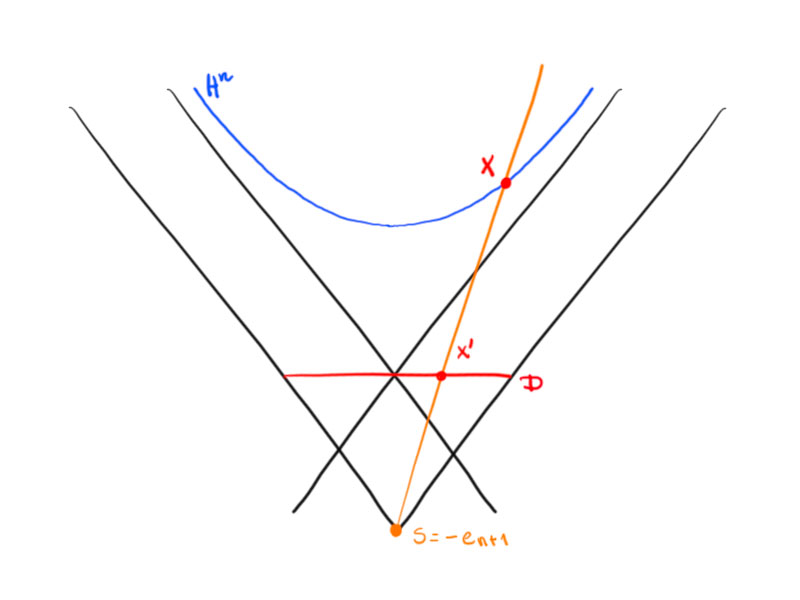
Consider the central projection with center $s$ of $H^n$ onto the plane $x_{n+1}=0$.
This map can be described by
\begin{align*}\sigma\colon H^n
&\to D=\{u\in\R^n:(u,u)<1\}\\
x&\mapsto\frac1{x_{n+1}+1}\begin{pmatrix} x_1\\\vdots\\x_n\end{pmatrix}\,.
\end{align*}
The inverse is given by
\[\sigma^{-1}(u)=\frac1{1-(u,u)}\begin{pmatrix} 2u\\1+(u,u)\end{pmatrix}\,.\]
For $s+t\left(\begin{pmatrix}u\\ 0\end{pmatrix}-s\right)=\begin{pmatrix}tu\\-1+t\end{pmatrix}$ is a point on $\vec{su}$ and
\[-1=\left\langle \begin{pmatrix}tu\\-1+t\end{pmatrix},\begin{pmatrix}tu\\-1+t\end{pmatrix}\right\rangle_{n,1}=t^2(u,u)-(t-1)^2=t^2(u,u)-t^2+2t-1\]
yields $t=0$ or $t(u,u)+2-t=0$ which is equivalent to $t=\frac2{1-(u,u)}$.
This implies $X=\begin{pmatrix}\frac2{1-(u,u)}u\\-1+\frac2{1-(u,u)}\end{pmatrix}=\frac1{1-(u,u)}\begin{pmatrix} 2u\\1+(u,u)\end{pmatrix}$.
The map $\sigma$ is the restriction of the following map to $H^n$:
\[x\mapsto s-\frac2{\langle x-s,x-s\rangle_{n,1}}(x-s)\,,\quad\text{for}\ \langle x-s,x-s\rangle_{n,1}\neq0\,.\]
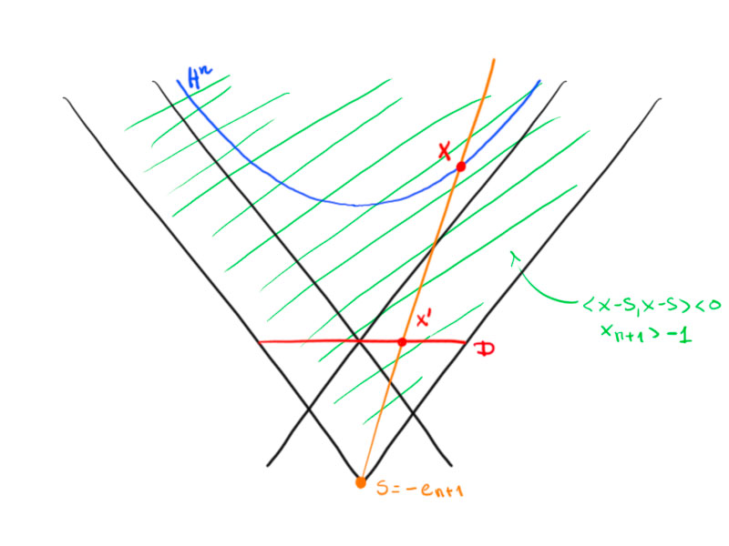
A point $x$ with $\langle x-s,x-s\rangle<0$ is mapped to a point on the ray $\vec{sx}$.
The plane $x_{n+1}=0$ is the orthogonal complement of $s$:
\begin{align*}\left\langle s-\frac2{\langle x-s,x-s\rangle}(x-s),s\right\rangle&=\langle s,s\rangle-\frac{2\langle x-s,s\rangle}{\langle x-s,x-s\rangle}=-1-\frac{2(\langle x,s\rangle-\langle s,s\rangle)}{\langle x,x\rangle-2\langle x,s\rangle+\langle s,s\rangle}\\&=-1-\frac{2(\langle x,s\rangle+1)}{-2-2\langle x,s\rangle}=0\,.\end{align*}
This map is an involution on the set $\{x\in\R^{n,1}:\langle x-s,x-s\rangle-1\}$ with $\sigma(H^n)=D$ and $\sigma(D)=H^n$, where $D\cong D\times\{0\}$.
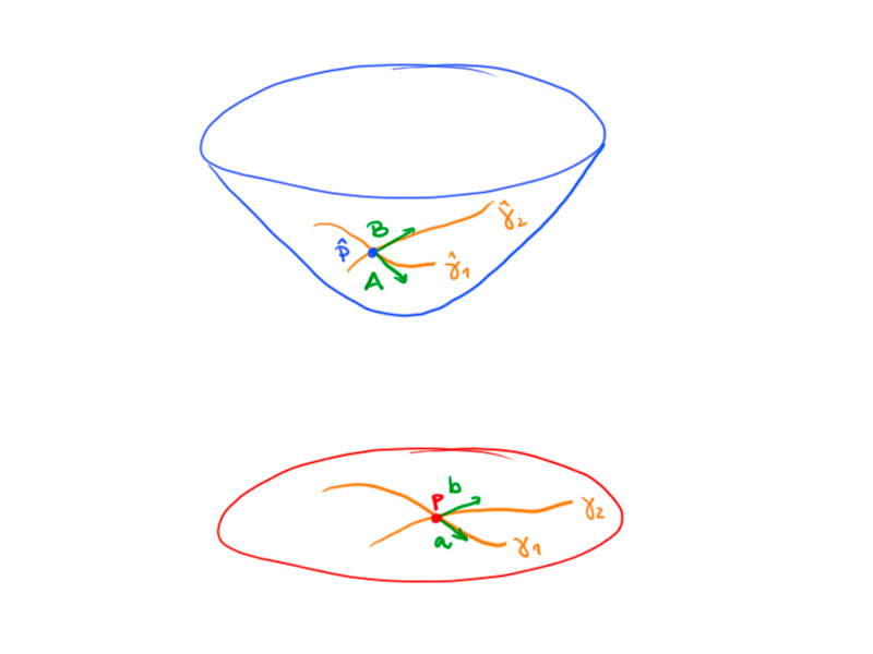
Theorem.
Consider two curves $\gamma_1,\gamma_2\subseteq D$ with $\gamma_1(0)=\gamma_2(0)=p\in D$ and $a:=\gamma_1′(0)$, $b:=\gamma_2′(0)$.
Let $\hat\gamma_1:=\sigma\circ\gamma_1$ and $\hat\gamma_2:=\sigma\circ\gamma_2$ be the corresponding curves in $H^n$ with $\hat\gamma_1(0)=\hat\gamma_2(0)=P=\sigma(p)$ and $A:=\hat\gamma_1′(0)$, $B:=\hat\gamma_2′(0)$.
Then:
\[\langle A,B\rangle_{n,1}=\frac4{(1-(p,p))^2}(a,b)\,.\]
This implies
\[\cosh\alpha=\frac{\langle A,B\rangle}{\sqrt{\langle A,A\rangle\langle B,B\rangle}}=\frac{(a,b)}{\sqrt{(a,a)(b,b)}}\,,\]
where $\alpha$ is the angle of intersection of $\hat\gamma_1$ and $\hat\gamma_2$.
Proof.
Calculate derivatives:
\[A=\hat\gamma_1′(0)=\frac{\mathrm d}{\mathrm dt}\left.\left(s-\frac2{\langle \gamma_1(t)-s,\gamma_1(t)\rangle}(\gamma_1(0)-s)\right)\right\vert{t=0}=-2\frac a{\langle p-s,p-s\rangle}+2\frac{2\langle p-s,a\rangle}{\langle p-s,p-s\rangle^2}(p-s)\,.\]
Similarly,
\[B=-2\frac b{\langle p-s,p-s\rangle}+2\frac{2\langle p-s,b\rangle}{\langle p-s,p-s\rangle^2}(p-s)\,.\]
Now,
\begin{align*}\langle A,B\rangle
&=\frac{4\langle a,b\rangle}{\langle p-s,p-s\rangle^2}-{2\cdot8\frac{\langle p-s,a\rangle\langle p-s,b\rangle}{\langle p-s,p-s\rangle^3}}+{16\frac{\langle p-s,a\rangle\langle p-s,b\rangle\langle p-s,p-s\rangle}{\langle p-s,p-s\rangle^4}}\\&=\frac4{(\langle p,p\rangle-2\langle p,s\rangle+\langle s,s\rangle)^2}(a,b)=\frac4{((p,p)-1)^2}(a,b)\,.\end{align*}
Definition
The open unit ball $D=\{u\in\R^n:(u,u)<1\}$ endowed with the \emph{Riemannian metric}
\[g_u(a,b)=\frac4{(1-(u,u))^2}(a,b)\,,\]
where $a$, $b$ are tangent vectors to $D$ at $u$, is the \emph{Poincaré ball model} of the hyperbolic space.
It is \emph{conformal}, i.e. the hyperbolic angles equal the Euclidean angles.
The \emph{length of a curve $\gamma\colon[0,1]\to D$} is given by
\[\operatorname{length}(\gamma)=\int_0^1\sqrt{g_{\gamma(t)}(\gamma'(t),\gamma'(t))}\mathrm dt\,.\]
Relation between Klein and Poincaré model
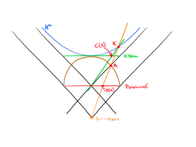
Claim: $A$ is the vertical projection along $e_{n+1}$ of $c(x)$ onto the hemisphere:
\[A_i=c(x)_i\quad\text{for all}\ i=1,\dotsc,n\,.\]
For this, observe that $A=s+t(x-s)$ for some $t$ and $(A,A)=1$.
Thus $\left(s+t\begin{pmatrix} x_1\\\vdots\\x_{n+1}+1\end{pmatrix},s+t\begin{pmatrix} x_1\\\vdots\\x_{n+1}+1\end{pmatrix}\right)=1$ yields
\[1=1+2\left(s,t\begin{pmatrix} x_1\\\vdots\\x_{n+1}+1\end{pmatrix}\right)+t^2\left\lVert\begin{pmatrix} x_1\\\vdots\\x_{n+1}+1\end{pmatrix}\right\rVert^2\]
and hence
\[0=-2t(x_{n+1}+1)+t^2\left(\sum_{i=1}^nx_i^2+x_{n+1}^2+2x_{n+1}+1\right)\,.\]
Now by $\langle x,x\rangle=-1$ we obtain
\[t^2\sum_{i=1}^nx_i^2=t^2(x_{n+1}^2-1)\]
which gives us $t=0$ or
\[t=\frac{2(x_{n+1}+1)}{2x_{n+1}(x_{n+1}+1)}=\frac1{x_{n+1}}\,.\]
So $A=\begin{pmatrix}0\\-1\end{pmatrix}+\frac1{x_{n+1}}\begin{pmatrix} x\\x_{n+1}+1\end{pmatrix}\in\R^{n,1}$.
Thus
\[(A)_{i=1,\dotsc,n}=\frac1{x_{n+1}}x\,.\]
The coordinates of $c(x)$ are given by
\[c(x)=\begin{pmatrix}\frac1{x_{n+1}}x\\1\end{pmatrix}\,.\]
This proves the claim.