If you have an exported png-image-sequence from jreality-export and you want make a h264-mp4 movie e.g. for embedding it to a website etc, you can use the following commands for it. Ensure that your files have straight enumerations (e.g. name000001.png – name999999.png) otherwise avidemux can not handle it.
Go to the image folder:
cd IMAGE_FOLDER
Use the convert “command” to make uncompressed jpg-files. This will also solve some colordepth issues for the movies later on:
for f in *.png; do
convert ./”$f” ./”${f%.png}.jpg”
done
Remove the png-files
rm *.png
Removes the commata from file-name [foo234,234.jpg -> foo234234jpg]
rename ‘s/,(\d{3})/$1/g’ *.jpg
Copies each 10th file to a subfolder
mkdir each10th
cp *0.jpg each10th/
cd each10th
Cuts the “0” (zero) at the end of the line. avidemux can just handle straight enumerations 00001-99999. (foo12340.jpg -> foo1234.jpg)
rename ‘s/(\d{3})([0]).jpg/$1.jpg/g’ *.jpg
Open the first file with avidemux -> Use as videocode “MPEG-4 AVC ” which is the H264-codec -> use as format mp4 ->press save and choose the location where to save -> done!
Comments Off on Convert jpg sequence to H264 mp4-movie with avidemux
If the given area $A$ is bigger than $4\pi$ and therefore bigger than a hemisphere we can’t use Euler rectangles anymore. Besides that the rest area is smaller than $4\pi, so we can cut the Sphere with 3 Euler Caps and will get a spherical rectangle without Euler restrictions: The areas we cut out will be rectangular to each other and corresponds to two Euler caps and one Euler rectangle.
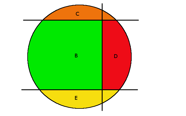
We consider now the following setup:
The area of the whole sphere is $8\pi$, the prescribed area $A$>4\pi$
The areas $C$ and $E$ have the same size $C=E<2pi$
If you cut a sphere with an arbitrary plane you will get a spherical cap. The spherical cap is either the region above or below that plane. There is one special case, when the plane passes through the center of the sphere. Then the cap is called hemisphere.
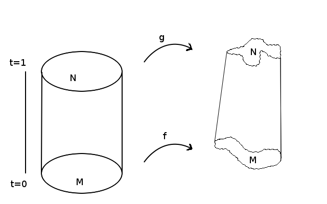
Def: Two immersions \(f\) and \(g\) are regularly homotopic if there exist a continuous family of immersions
\(f_t : M \rightarrow \mathbb{R}^n, t \in [0,1]\) such that \(f_0 = f\) and \(f_1 = g\)
Def: A regular homotopy between two immersions \(f\) and \(g\) from a Manifold \(M\) to a manifold \(N\) is defined to be a differentiable function \(H: M \times [0,1] \rightarrow N \) such that for all \(t \in [0,1]\). The Function \(H_t: M \rightarrow N\) defined by \(H_t(x)=H(x,t) \forall x \in M\) is an immersion, with \(H_0 = f\) and \(H_1 = g\). A regular homotopy is thus a homotopy through immersions.
As far as I understand this is cobordism as well
Further I’m wondering how many homotopy-classes exist. Ulrich wrote in his paper:
If $M^2$ is a compact surface, $h = \dim H_1(M^2, \mathbb{Z}_2)$ then the space $ I(M^2, \mathbb{R}^3)$ of immersions $f: M^2 \rightarrow \mathbb{R}^3$ has $2^h$ connected components.
Is $2^h= 2^{(2^g)}$ what Keenan suggested?
In an other paper I found that the number ob homotopy classes is $4^g$
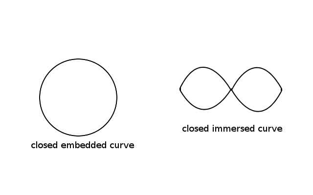
Def: A surface \(M\) is \(n\)-embeddable if it is not self-intersecting, placed in an \(mathbb{R}^n\)-space. An self-intersecting surface can be called an immersion. Further all embeddings are immersions, but not the other way around.
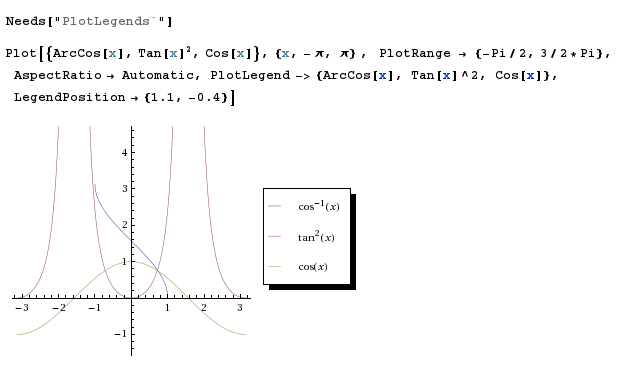
where \(\gamma\) is the angle and \(w,h\) correspond to width and height of the rectangle. If we want to determine all lengths and areas we cover with spherical rectangles we have to check the above formulas for their borders. If we focus on the formula for the width we have to examine three trigonometrical functions \((\arccos(x), \tan^2 (x), \cos(x))\).
\(\cos(x)\) is defined anywhere
\(\tan^2(x)\) is not defined at multiples of \(\pm \pi/2 \)
\(\arccos(x)\) is just defined between \(-1\) and \(1\)
also displayed in the figure below:
So we have to solve the \(\arccos(x)\) in between \(-1\) and \(1\)
The inequality changes because \(\arccos\) is strictly monotonic decreasing \((x<y \rightarrow \arccos x > \arccos y)\). In the next step we substitute \(\frac {\gamma}{2}=\frac{A}{8} + \frac{\pi}{4}\).
The inequality above would be the solution for an \((A,L)\)-diagram, but we are interested in half the area \(a=A/2 \rightarrow 2a = A\) and the same for the length \( l= L/2 \rightarrow 2l = L \) so we get
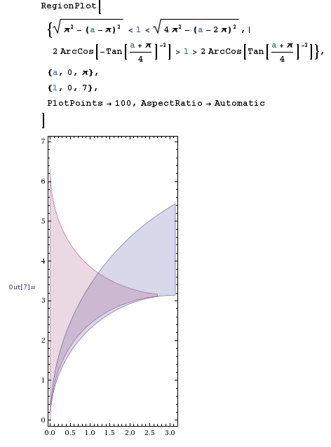
Ulrich wrote in his article about the conformal structure: ” If the conformal structure is not rectangular then we chose a corresponding point \((A,L)\) in the region \(U \subset \mathbb{R}^2 \) defined by the inequalities
Plotting these two areas corresponds to the figure below. The blue area is the requested conformal structure and the red one, the area for the rectangles. So we can at least represent the tori with almost rectangular structure. So for the start we can work with rectangles but we have to search an other spherical curve which covers the full “blue” area.
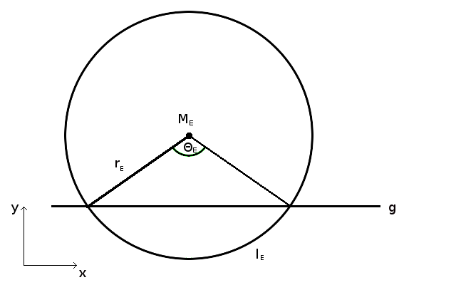
We just figured out, that we can’t deal with Euler geometry on spheres to cover the hexagonal tori parts of the \(A/2\) / \(L/2\) diagram. With Euler rectangles the biggest area \(A= 2\pi\) and the same for the length \(L=2\pi\). But Ulrich deals in his paper also with hexagonal tori, whose length \(L= \sqrt 3 \cdot 2\pi\) is bigger than \(2 \pi\).
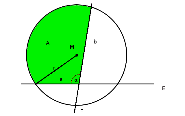
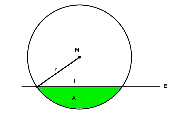
Therefore we skipped the rectangle and started to focus on spherical arcs, which aren’t based on big circles. The construction is simple, just add to planes \((E, F)\) to the sphere, that the length \(L\) is \(L =a+b\) and the area \(A\) is a linear combination of \( a, b, \alpha\), which I haven’t calculated yet. The figure below visualizes such a construction.
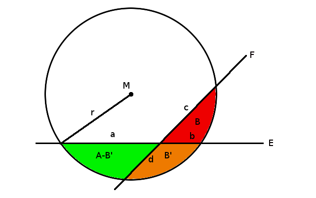
As I was thinking about the problem I just figured out, that Ulrich is doing something similar with his intersecting double-disk construction. He first draws a plane \(E\) fixing the area \(A\).
Then he draws a second plane \(F\) such that the orange area \(B’\) and the red area \(B\) have the same size \(B’=B\) and therefore the total area \(A = green + red\) is unchanged. The length \(L\) can further be determined by \(L=a+b+c+d\)
Hamilton invented in 1843 quaternions \(\mathbb{H}\) to deal easier with rotations in \(\mathbb{R}^3\). As a set, the quaternions \(\mathbb{H}\) are identical to \(\mathbb{R}^4\) (four-dim vector space over real numbers). To deal with \(\mathbb{H}\) in \(\mathbb{R}^4\) we define a basis denoted as \(1, i, j, k \). Every quaternion can be written as a combination of the basis times a real variable, \(a1 +bi, + cj + dk\), where \(a,b,c,d\) are the real variables. Further \(1\) denotes the identity of \(\mathbb{H}\)
Multiplication of basis elements:
\[\begin{array}{} i^2 = & j^2 = & k^2 = & ijk = -1 \\ ij = k & jk = i & ik = j \\ ji = -k & kj = -i & ki = -j \end{array}\]
With the basis \(1, i, j, k \), \(\mathbb{H}\) can be written as set of quadruples:
When \(q\) is an unit quaternion \(q^{-1}=\bar q\).
Given two unit quaternions \(p = xi+yj+zk, q = x’i+ y’j+z’k\). The quaternionproduct \(qpq^{-1}\) rotates the vertex \(v=(x,y,z)\) to \(v’= (x’,y’,z’)\) and can be defined as a map \(R_q: \mathbb{R}^3 \rightarrow \mathbb{R}^3 \). For \(q \neq 0, R_q\) is a rotation of \(\mathbb{R}^3\), where the axis and the angle are described by the four coordinates \((a,b,c,d)\) in the following way. If \(q = +-1\), \(R_q\) is the identity mapping on \(\mathbb{R}^3\). Otherwise \(R_q\) ist a rotation about the axis determined by the vector \((b,c,d)\).