Let $M= \left(V, E, F \right)$ be an oriented triangulated surface without boundary and $p:V \rightarrow \mathbb{R}^3$ a realization. In earlier lectures we considered the space of piecewise linear functions on $M$:
\[W_{PL}:=\left\{ \tilde{f} :M\rightarrow \mathbb{R} \, \big \vert \,\left. \tilde{f}\right|_{\sigma} \mbox{ is affine for all } \sigma \in F \right\}.\]
A basis of $W_{PL}$ is given by : $\phi_i \in W_{PL}$ defined by $\phi_i(p_j) = \delta_{ij},$ an interpolation map is defined by:
\begin{align*} \mbox{int}_{PL} : \mathbb{R}^{V} & \rightarrow W_{PL}, \\
f & \mapsto \tilde{f} = \sum_{i \in V} f_i \phi_i.
\end{align*}
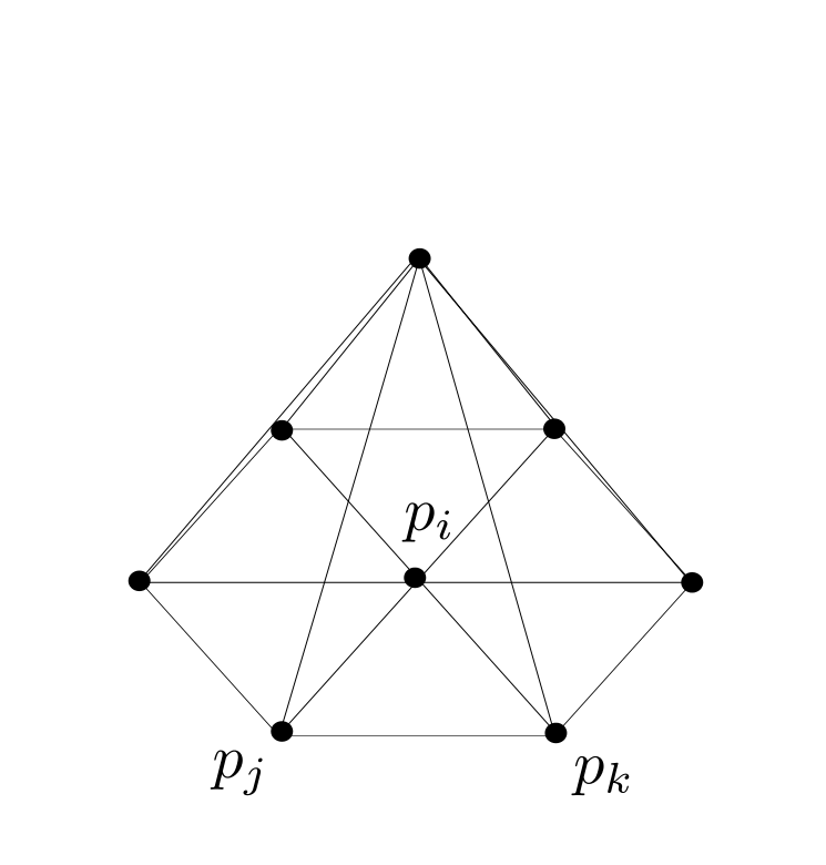
The graph of $\phi_i$
For some purposes piecewise constant function are more convenient then piecewise linear ones, therefore, we introduce a new function space on $M$ that consists of piecewise constant functions. In order to do that we assign a domain to each vertex:
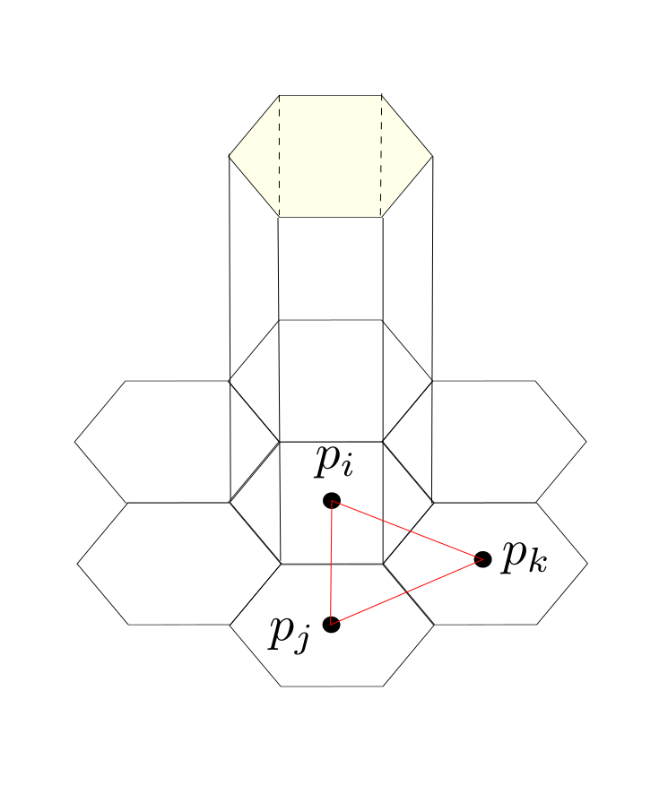
For every edge $e_{ij} \in E$ the center is given by $S_{ij}= \frac{1}{2}\left( p_i + p_j \right)$ analog for every triangle $\sigma = \{i,j,k\} \in F$ the center of mass is defined as $S_{ijk} = \frac{1}{3} \left( p_i + p_j + p_k\right) $.
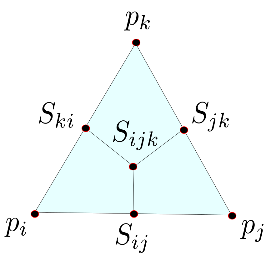
If we connect the center of the edges with the center of mass the triangle is divided into three parts with equal area. Now we can assign to each vertex $p_i$ the parts of the adjacent triangles that contain $p_i$ and denote it with $D_i$.
The domain $D_i$ (gray colored) associated to the vertex $p_i$
For the area of $D_i$ we obtain:
\[A_i := \frac{1}{3} \sum_{ \sigma = \{i,j,k\} \in F} A_{\sigma}. \]
The space of piecewise constant functions is defined in the following way:
\[W_{PC}:= \left\{\hat{f} :M \rightarrow \mathbb{R} \, \big \vert \, \left. \hat{f}\right|_{D_i} \mbox{ is constant for all } i \in V \right\}.\]
Also on $W_{PC}$ we have a canonical basis $\Psi_i \in W_{PC}$ defined by $\Psi_i(p_j) = \delta_{ij} $ and an interpolation map:
\begin{align*} \mbox{int}_{PC} : \mathbb{R}^{V} & \rightarrow W_{PC}, \\
f & \mapsto \hat{f} = \sum_{i \in V} f_i \Psi_i.
\end{align*}
Graph of $\Psi_i$
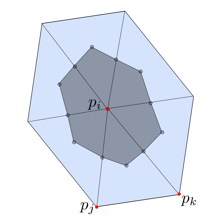
There is a similar construction that assigns to each vertex an face and works purely combinatorial: For a triangulated $M$ surface one can define its discrete dual surface $M^{\ast}=\left( V^{\ast},E^{\ast},F^{\ast}\right)$. The faces of $M$ correspond to the vertices of $M^{\ast}$ and the vertices of $M$ to the faces of $M^{\ast}$. The set of edges stays the same. Two vertices in $M^{\ast}$ are connected by an edge if the corresponding faces in $M$ are adjacent. For more informations see here.
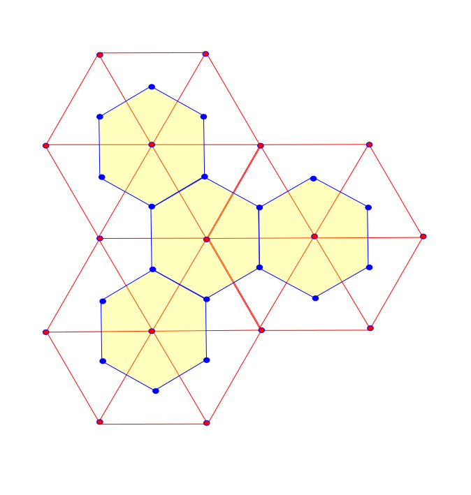
A piece of an triangulated surface $M$ and its dual $M^{\ast}$. The red vertices and edges belong to $M$ and the blues ones to $M^{\ast}$.
Since in general it is not easy to compute the area of the dual faces with the metric of the original one, we used the above construction of the $D_i$’s to define $W_{PC}$. On $W_{PL}$ we defined the usual scalar product $ \langle\!\langle \tilde{f}, \tilde{g} \rangle\!\rangle_{PL} := \int_M \tilde{f}\tilde{g}$ and computed the matrix $B$ representing it with respect to the basis $\left\{ \phi_1,\ldots \phi_N \right\},$ i.e. $b_{ij}:=\langle\!\langle\phi_i, \phi_j \rangle\!\rangle_{PL}.$ This gave us a scalar product on $\mathbb{R}^V$:
\[\langle\!\langle f, g \rangle\!\rangle_{PL} = f^tBg = \sum_{i,j \in V} f_i g_j b_{ij}.\]
On the same way we define an scalarproduct on $W_{PC}$:
\begin{align*}\langle\!\langle\cdot, \cdot \rangle\!\rangle_{PC} &: W_{PC}\times W_{PC} \rightarrow \mathbb{R}, \\ \langle\!\langle \hat{f}, \hat{g} \rangle\!\rangle_{PC} & := \int_M\hat{f}\hat{g}.\end{align*}
The matrix $A$ representing it with respect to the basis $\left\{ \Psi_1,\ldots \Psi_N \right\}$ is a diagonal matrix since:
\[a_{ij}:=\langle\!\langle\Psi_i, \Psi_j \rangle\!\rangle_{PC}\ = \int_M \Psi_i \Psi_j = A_i \delta_{ij}.\]
This gives us a new scalar product on $\mathbb{R}^V:$
\[\langle\!\langle f, g \rangle\!\rangle_{PC} := f^tAg = \sum_{i \in V} f_i g_i a_{ii}.\]
Note that the basis $\left\{ \Psi_1,\ldots \Psi_N \right\}$ is orthogonal with respect to $\langle\!\langle \cdot, \cdot \rangle\!\rangle_{PC}$, while the same is not true for $\left\{ \phi_1,\ldots \phi_N \right\}$ with respect to $\langle\!\langle \cdot, \cdot \rangle\!\rangle_{PL}$.
Now we have two scalar products on $\mathbb{R}^V$ one represented by a symmetric positive definite matrix $B$ and one by a positive definite diagonal one $A$.
Our aim is to define a discrete laplace operator $\Delta:\mathbb{R}^V \rightarrow \mathbb{R}^V$ analog to the smooth laplacian we discussed earlier. We will see that the discrtelaplacian depends on the choice of scalarproduct.
On a smooth surface $M$ we have:
\[\langle\!\langle \Delta f, g \rangle\!\rangle = \int_M \Delta f g =\, – \int_M \langle \mbox{grad}\, f , \mbox{grad}\, g \rangle.\]
This identity should also be true in the discrete case and will serve us as definition for the discrete laplacian. We already defined the bilinear operator
\begin{align} L: \mathbb{R}^V \times \mathbb{R}^V & \rightarrow \mathbb{R},\\ f,g & \mapsto \, – \int_M \langle \mbox{grad}\, f , \mbox{grad}\, g \rangle ,\end{align}
and discussed the relation between quadratic forms, symmetric bilinear maps and maps between dual spaces ( lecture: dirichlet energy 2 ).
\[\begin{array}{lcl} W_{PL} & \overset{E_D}{\longrightarrow} & W_{PL}^{\ast} \\ \uparrow \mbox{interpol.} & & \downarrow \mbox{interpol.}^{\ast} \\ \mathbb{R}^V & \overset{L}{\longrightarrow} & \mathbb{R}^{V\ast} \end{array} \]
In the finite case the quadratic form, bilinear form and map between the dual spaces can all be represented by the same matrix $L$ .
For $f,g \in \mathbb{R}^V$ we have:
\[f^tLg = \,- \int_M \langle \mbox{grad}\, f , \mbox{grad}\, g \rangle\overset{!}{=} \int_M \Delta f g = \langle\!\langle \Delta f, g \rangle\!\rangle .\]
This gives us one laplace operator for each scalarproduct on $\mathbb{R}^V$:
\begin{align} f^tLg = \left\{ \begin{array} {cc} \left(\Delta_{PL} f\right)^tBg, \\ \left(\Delta_{PC} f\right)^tAg,\end{array} \right. \\ \Rightarrow \left\{ \begin{array} {cc} \Delta_{PL} = \left(LB^{-1} \right)^t = B^{-1}L , \\ \Delta_{PC} = \left(LA^{-1} \right)^t = A^{-1}L. \end{array} \right. \end{align}
In general it is complicated and expensive to compute $B^{-1}$, such that it is much easier to use $\Delta_{PC}$ instead of $\Delta_{PL}$. Witch of the laplacians one has to choose depends on the nature of the problem.
One famous problem form physics and geometry is the Poisson problem:
Given $\rho \in \mathbb{R}^V$ find $u \in \mathbb{R}^V$ such that:
\[\Delta \,u = -\rho.\]
For Poisson problems both laplacians can be used since:
\[\Delta_{PL} u = \left(LB^{-1} \right)^t u = \,- \rho \Leftrightarrow Lu = -B\rho. \]
Example: Suppose $M$ consists of an uniform conducting material and $\rho: M \rightarrow \mathbb{R}$ is a charge density. For the electric field $E$ on $M$ there holds:
\[\mbox{div} E = \rho,\]
and for the potential $u: M \rightarrow \mathbb{R}$ we have
\[E=-\mbox{grad}\, u.\]Taking this together we have to solve:
\[\Delta \,u = -\rho,\]
in order to determine the potential for a given density.
In this setting piecewise constant functions are much more convenient to describe the charge density then piecewise linear ones. Therefore we use $\Delta_{PL} $ to solve this problem.