Tutorial 12: The Pendulum

A pendulum is a body suspended from a fixed support so that it swings freely back and forth under the influence of gravity. A simple pendulum is an idealization of a real pendulum—a point of mass $m$ moving on circle of radius $\ell$ under the influence of a uniform uniform gravity field of strength $g$ pointing down.

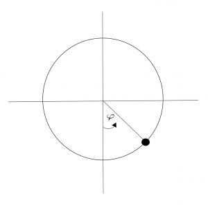
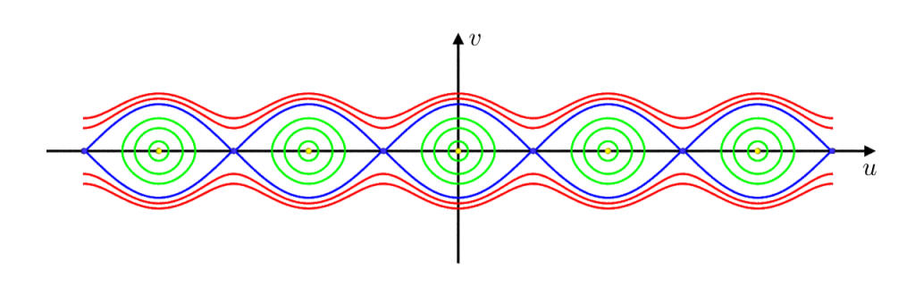
Its position is described by an angular coordinate $\phi$ and its energy is the sum of  kinetic energy $\frac{m}{2}{\ell }^2{\dot{\phi }}^2$ and gravitational potential energy  $-m\ell g\cos \phi$:$$E(\phi ,\dot{\phi })=\frac{m}{2}{\ell }^2{\dot{\phi }}^2–m\ell g\cos \phi .$$Its motion is then described by the following differential equation: $$\ddot{\phi }=-\frac{g}{\ell }\sin \phi .$$One easily checks that energy is a constant of motion,$$\dot{E}=m{\ell }^2\dot{\phi }\ddot{\phi }+m\ell g\dot{\phi }\sin \phi =-m\ell \dot{\phi }g\sin \phi +m\ell g\dot{\phi }\sin \phi =0.$$ Here a picture of the corresponding energy levels in phase space.

In the following we will set $m=g=\ell =1$.

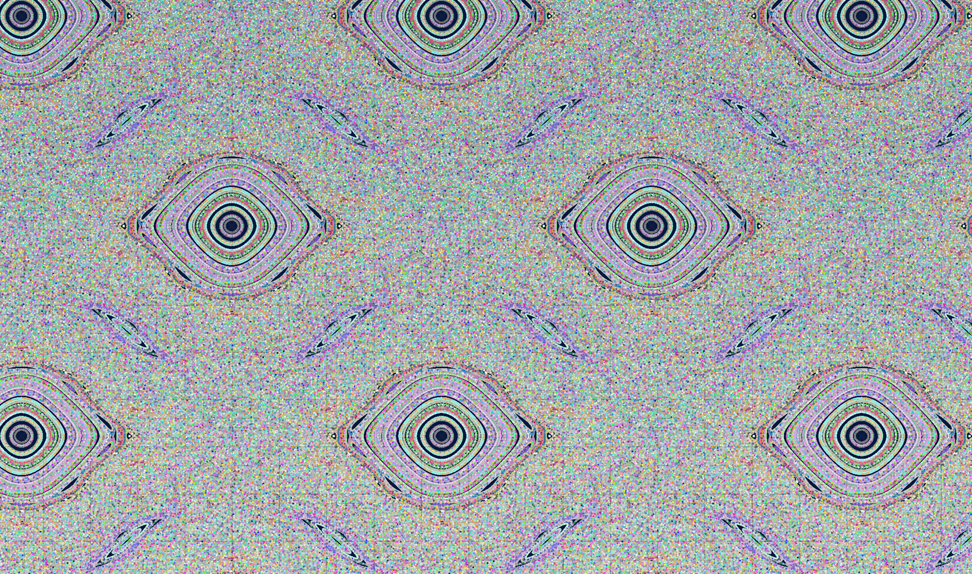
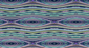
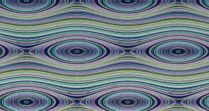
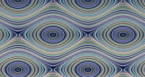
The simple pendulum is what is called an integrable Hamiltonian system. Now, if we discretize $\ddot{\phi }$ with timestep $\epsilon >0$ according to the Verlét we obtain the following recursion:$$\left(\begin{array}{c}{\phi }_{n+1}\\ {\phi }_n\end{array}\right)=\sigma \left(\begin{array}{c}{\phi }_n\\ {\phi }_{n-1}\end{array}\right)\mathrm{mod}2\pi {\mathbb{Z}}^2,$$where $\sigma :{\mathbb{R}}^2\to {\mathbb{R}}^2$ is given by$$\sigma \left(\begin{array}{c}{\phi }_n\\ {\phi }_{n-1}\end{array}\right):=\left(\begin{array}{c}2{\phi }_n–{\phi }_{n-1}–K\sin ({\phi }_n)\\ {\phi }_n\end{array}\right),K={\epsilon }^2.$$The map $\sigma$ is the well-known Chirikov standard map—an area-preserving (i.e. symplectic) map, which shows chaotic behavior. As such it serves as an important model in chaos theory.

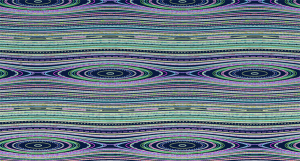
Here $K=0.2,0.5,0.7,0.9$ from top to bottom.

The phase space is not ordered anymore by the constants of motion. Though order is not totally gone. The chaotic regions cannot diffuse over the whole phase space but are bounded by so-called KAM orbits. As guaranteed by Kolmogorov–Arnold–Moser (KAM) theory, a non-neglectable amount will survive for small perturbations.

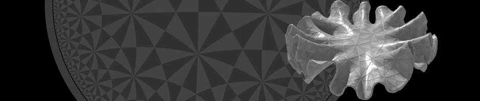
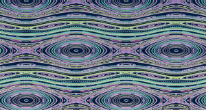
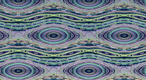
Remarkably, if we use $4\arg (1+K{e}^{-i\phi })$ instead of $\sin \phi$ in the iteration we again obtain an integrable system. How to get to this discrete version of $\sin$ in this article. It also provides a formula for the constant of motion.

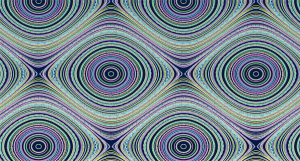
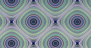
Here again $K=0.2,0.5,0.7,0.9$ from top to bottom.

To produce these pictures in Houdini one can just randomly seed a bunch of particles on a the square $M=[-\pi ,\pi {]}^2$, color it randomly and iterate by a solver node. To visualize the whole sequence one can keep track of the history using a trail node. Though if we want to play around with parameters that is not an optimal setup. One better uses a loop with feedback—only one has to remember the point positions in each iteration.

Here is a way to do this: In the $(k+1)$st iteration we extract the points of the $k$th iteration by a delete node. Then we apply the iteration formula and merge again with all previous points. Since the merge node just appends the points we can extract using a delete node. The network thus might look as follows.

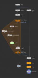
The copy and transform nodes at the end are used to copy the fundamental domain in $x$- and $y$-direction—just for visualization purposes.

Homework (due 9 July). Build a network that visualizes the orbits of the pendulum equation. It shall be possible to specify $K$, the number of orbits and the total number of iterations (resolution of the obits). Use a checkbox parameter to choose between $\sin$ and its discrete counterpart.