In this very first tutorial we will describe how to solve initial value problems using Houdini. We will first play this through for an first order ODE – the Lorenz system – before you apply the solver to compute the trajectories of charged particles in a static magnetic field.
Consider a smooth vector field
The most naive way to numerically approximate a solution is to successively perform linear steps along the tangent. This leads to the so called Euler method: For a given small time step
Certainly, we cannot expect high accuracy. E.g., if
The Euler method is easily implemented using Houdini’s Solver node. Here is how such a network may look like (inside a geometry node):
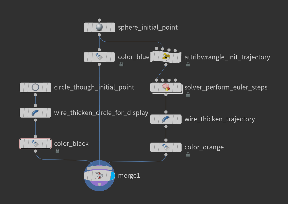
The Attribute Wrangle node “init trajectory” just takes the initial point (center of a sphere primitive) and turns it in an open polygon (polyline):
The Euler step is performed inside a solver node. Let us dive into the solver node:
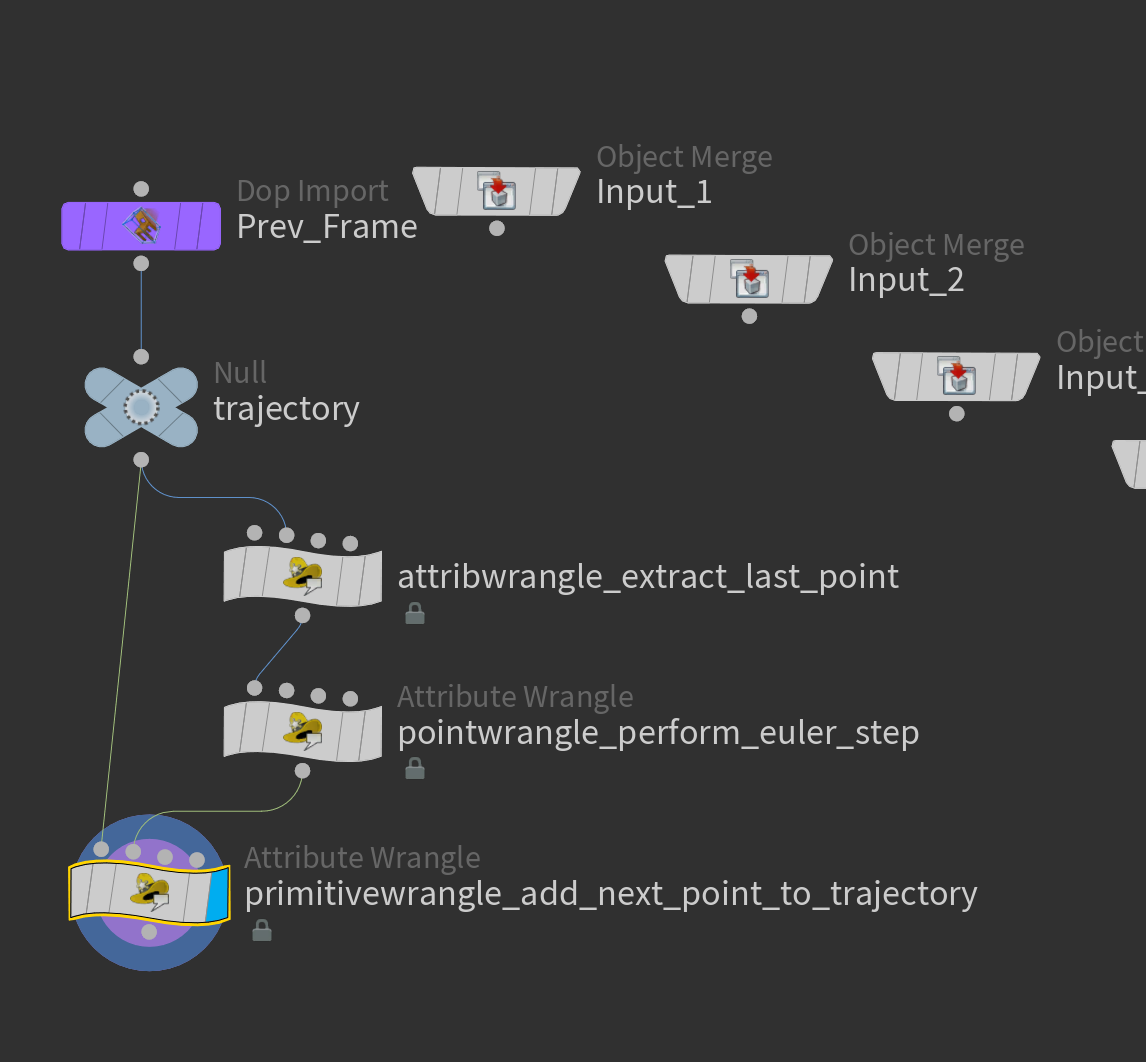
Here we use an Attribute Wrangle node (which ‘runs over’ detail) to extract the last point of the trajectory curve,
perform an Euler step (Point Wrangle node).
and add this point to the trajectory curve (Primitive Wrangle node)
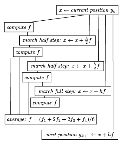
A more sophisticated method to solve differential equations is the so called Runge-Kutta method (RK4) It basically consists of 4 Euler steps and schematically this looks as follows:
The scheme translates one to one into a Houdini network which then replaces the single Euler step node of the previous network:
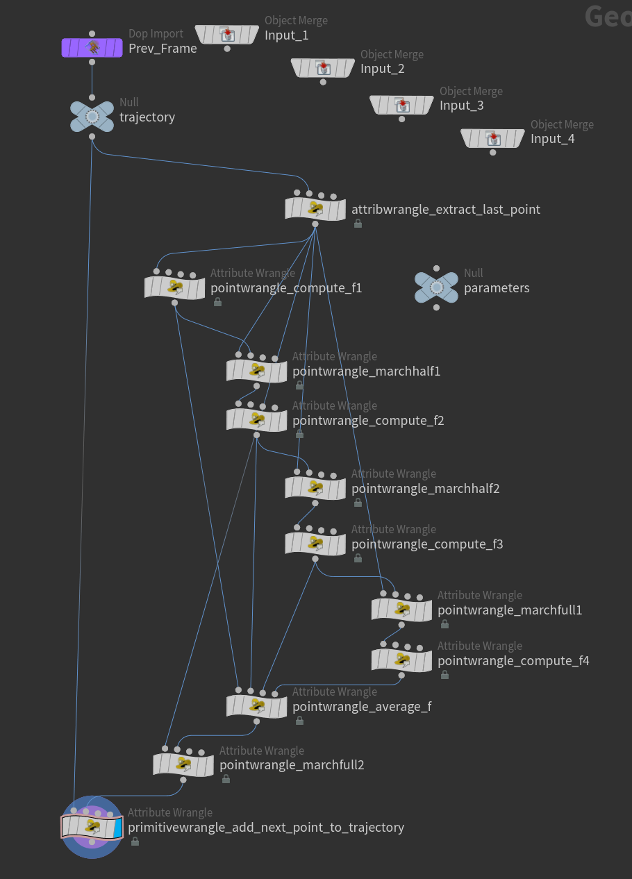
Moreover, we used here a null node to store the step size as a float parameter
Similarly the ‘compute f’ nodes even consist of just one line
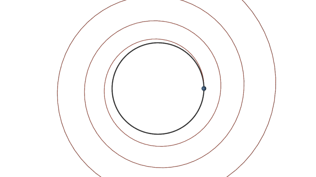
With the RK4 method we then obtain for
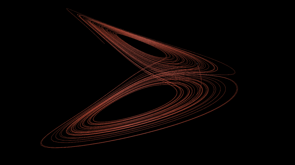
Let us apply this to the Lorenz attractor. We only have to change
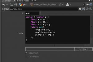
The code written there then can be imported in wrangle nodes by inserting <code>chs("../parameters/code") at the start of the ‘VEXpression’ field. E.g.
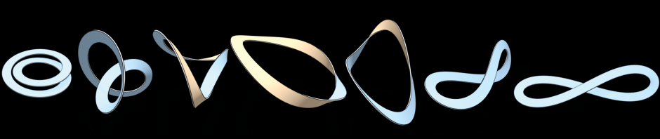
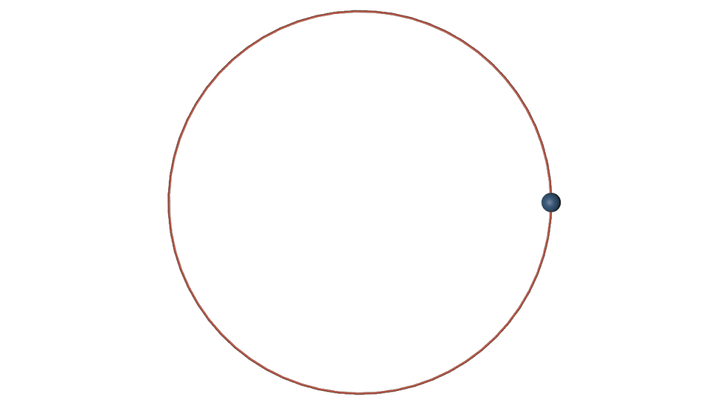
Here how the result then may look like:
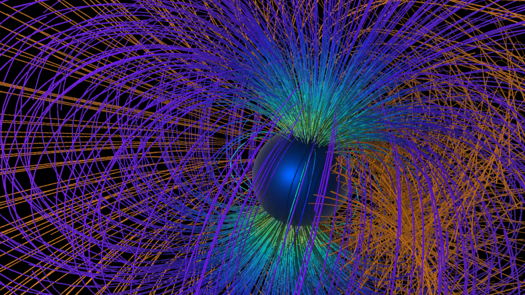
The motion of a particle of charge
Homework (due 8 May). Modify the network such that it computes the trajectory of a charged particle moving in the field of a magnetic dipole. Therefore change the RK4 solver such that it operates on a float[] point attribute
Further one can use a Scatter node to generate particles equally distributed on a given geometry. Here a picture of 500 particles (with constant initial velocity) shot at a magnetic dipole.