Conformal Maps II: Inversions

Let $M\subset \mathbb{R}^n$ be a domain. A smooth map $f:M \to \mathbb{R}^n$ is called conformal if there is a smooth function $\phi:M\to \mathbb{R}$ and a smooth map $A$ from $M$ into the group $O(n)$ of orthogonal $n\times n$-matrices such that the derivative $f’$ of $f$ satisfies

\[f’=e^\phi A.\]

In the two dimensional case this definition agrees with the one given in an earlier post. It means that when restricting attention to very small regions (i.e. looking through a microscope) $f$ looks like a similarity transformation. The similarity transformations themselves, defined as affine maps of the form

\begin{align*}f:\mathbb{R}^n &\to \mathbb{R}^n \\\\ f(\mathbf{x}) &=e^\phi A \mathbf{x}+\mathbf{b}\end{align*}

with $\phi\in\mathbb{R}$, $A\in O(n)$, $\mathbf{b}\in\mathbb{R}^n$ are standard examples of conformal maps.

The theory of holomorphic functions shows that for $n=2$ there is an abundance of conformal maps $f$ from domains in $M\subset \mathbb{R}^n$ into $\mathbb{R}^n$. In contrast, a famous theorem proved by Liouville in 1850 says that for $n \geq 3$ all such maps $f$ are of the form

\[f= s_1\circ g \circ s_2\]

where $s_1$ and $s_2$ are similarity transformations and

\begin{align*}g:\mathbb{R}^n\setminus\{\mathbf{o}\} &\to \mathbb{R}^n\setminus\{\mathbf{o}\} \\\\ g(\mathbf{x}) &=\frac{\!\!\!\mathbf{x}}{|\mathbf{x}|^2}\end{align*}

is the so-called inversion in the unit sphere $S^{n-1}$. Inversion interchanges the exterior of $S^{n-1}$ with its interior (from which the origin has been removed). All points of $S^{n-1}$ are fixpoints of $g$. For this reason $g$ is also called the reflection in the unit sphere.

Let us prove that $g$ is conformal. For all $\mathbf{x}\in\mathbb{R}^n\setminus\{\mathbf{o}\}$ and $\mathbf{y}\in \mathbb{R}^n$ we have

\begin{align*}g'(\mathbf{x})\,\mathbf{y}&=\frac{\!\!\!\mathbf{y}}{|\mathbf{x}|^2}-\frac{2\langle \mathbf{x},\mathbf{y}\rangle}{|\mathbf{x}|^4}\\\\ &=\frac{\!\!\!1}{|\mathbf{x}|^2}\left(\mathbf{y}-2\left\langle \frac{\mathbf{x}}{|\mathbf{x}|},\mathbf{y}\right\rangle\frac{\mathbf{x}}{|\mathbf{x}|}\right).\end{align*}

Now the map

\[\mathbf{y} \mapsto A\mathbf{y}:=\mathbf{y}-2\left\langle \frac{\mathbf{x}}{|\mathbf{x}|},\mathbf{y}\right\rangle\frac{\mathbf{x}}{|\mathbf{x}|}\]

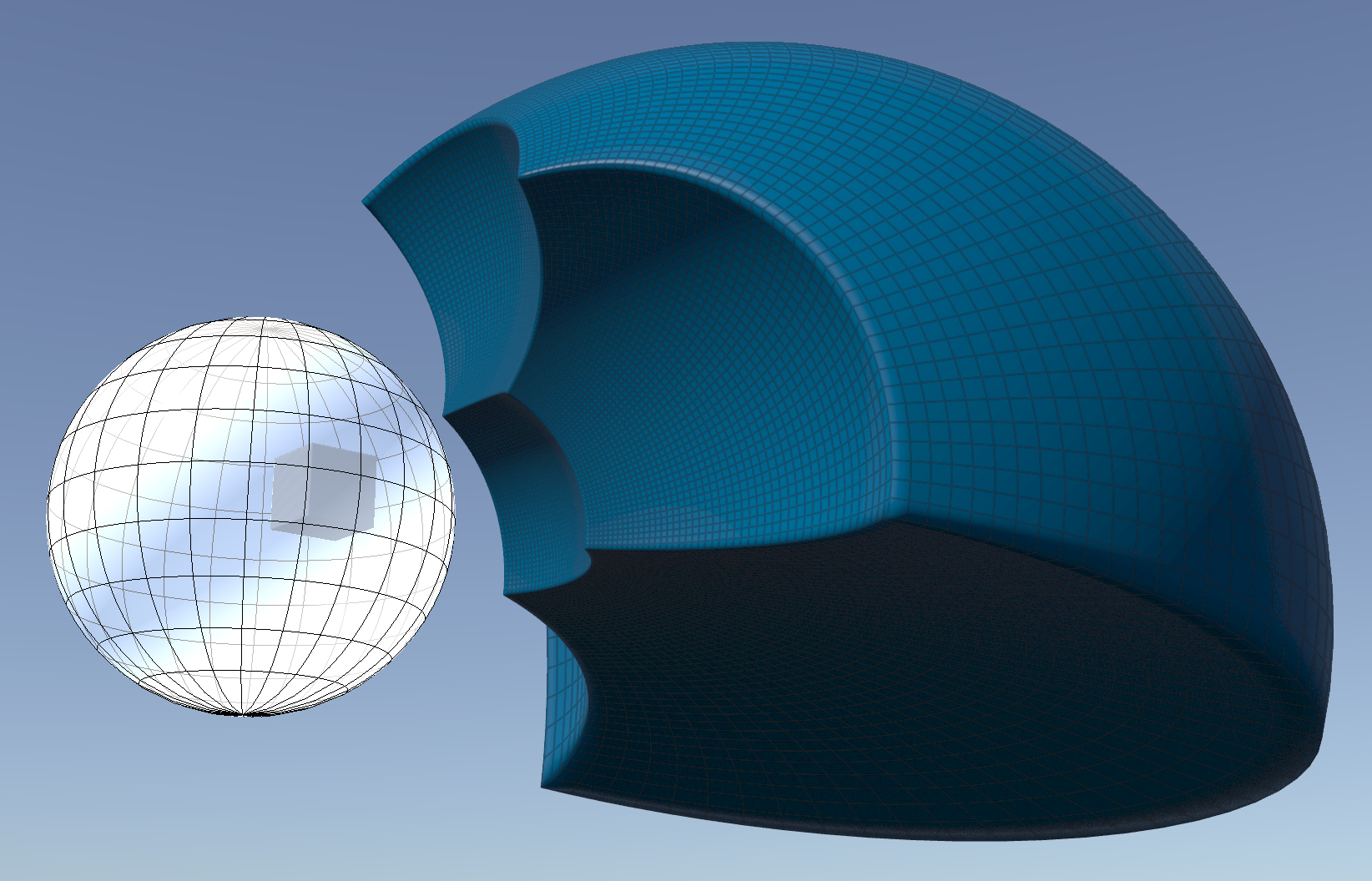
is reflection in the unit vector $\frac{\mathbf{x}}{|\mathbf{x}|}$ and therefore orthogonal. Thus $g$ is conformal. Here is what happens if we apply $g$ to a small cube inside the unit sphere:

 inversion-3

Apparently, all cube faces are mapped to pieces of round spheres. Let us prove this in general: If we have a hyperplane

\[E = \{\mathbf{x}\in \mathbb{R}^n \,|\,\langle \mathbf{x},\mathbf{n}\rangle = d\}\]

with unit normal $\mathbf{n}$ and distance $d\neq 0$ to the origin, then all points $\mathbf{x}\in g(E)$ satisfy

\begin{align*}0&=\left\langle\frac{\!\!\!\mathbf{x}}{|\mathbf{x}|^2},\mathbf{n}\right\rangle -d\\\\&=-\frac{\!\!\!d}{|\mathbf{x}|^2}\left(\left\langle \mathbf{x} -\frac{\mathbf{n}}{2 d},\mathbf{x}-\frac{\mathbf{n}}{2 d}\right\rangle -\frac{1}{4 d^2}\right).\end{align*}

So they lie on the sphere with center $\frac{n}{2d}$ and radius $\frac{2d}$. A similar computation shows that any piece of a sphere or plane that does not contain the origin is mapped onto a piece of another sphere or plane. Since planes can be regarded as limiting cases of spheres, a concise though slightly sloppy way to express this fact is by saying that “$g$ transforms spheres into spheres”.

The inversion in a sphere with center $\mathbf{m}$ and radius $r$ is defined as

\[\mathbf{y}\mapsto \mathbf{m}+\frac{\!\!\!\mathbf{y}-\mathbf{m}}{\left|\mathbf{y}-\mathbf{m}\right|^2}.\]

Posted in Lecture | Comments Off on Conformal Maps II: Inversions

Quaternions

Quaternions, $\mathbb{H}$ are a number system like real or complex numbers but with 4 dimensions. In particular, $\mathbb{H}$ is nothing but $\mathbb{R}^4$ together with a multiplication law. The identification of $\mathbb{H}$ and $\mathbb{R}^4$ is given by:
$$ \mathbb{H} = \lbrace x_0 + x_1 {\bf i} + x_2 {\bf j} + x_3 {\bf k} \,\vert \,x_0,x_1,x_2,x_3 \in \mathbb{R} \rbrace.$$
With the usual addition and scalar multiplication inherited from $\mathbb{R}^4$, $\mathbb{H}$ becomes a four dimensional  $\mathbb{R}$ vector space with canonical basis $\{ 1, {\bf i}, {\bf j}, {\bf k} \}.$ The quaternion multiplication is defined by:
\begin{align*}
&\left(x_0 + x_1 {\bf i} + x_2{\bf j} + x_3 {\bf k} \right) \cdot \left(y_0 + y_1{\bf i} + y_2{\bf j} + y_3  {\bf k} \right) \\:= & \left(x_0 y_0 – x_1 y_1 – x_2 y_2 – x_3 y_3 \right) \\
+ & \left(x_0 y_1 + x_1 y_0 + x_2 y_3 – x_3 y_2 \right){\bf i} \\
+ & \left(x_0 y_2 – x_1 y_3 + x_2 y_0 + x_3 y_1 \right){\bf j} \\
+ & \left(x_0 y_3 + x_1 y_2 – x_2 y_1 + x_3 y_0 \right) {\bf k}.
\end{align*}

A more simple way to define the quaternion multiplication is to say that the multiplication with $\alpha \in \mathbb{R}$ works as usually and that ${\bf i}, {\bf j}, {\bf k}$ satisfy the following  multiplication rules:

\[{\bf i}^2 = {\bf j}^2 = {\bf k}^2 = -1,\quad {\bf ij}=-{\bf ji}={\bf k}, \quad {\bf jk}=-{\bf kj}={\bf i}, \quad {\bf ki}=-{\bf ik}={\bf j}.\]

${\rm Re}(\mathbb{H}) := span\{1\}$ is called the real part of  $\mathbb{H}$ and ${\rm Im}(\mathbb{H}) := span\{{\bf i}, {\bf j}, {\bf k}\}$  the imaginary part and there holds:  $\mathbb{H} = {\rm Re}(\mathbb{H}) \oplus {\rm Im}(\mathbb{H})$. If we identify ${\rm Re}(\mathbb{H})$ with $\mathbb{R}$ and ${\rm Im}(\mathbb{H})$ with $\mathbb{R}^3$, we can write any ${\bf x} \in \mathbb{H} $ as: $\quad {\bf x} = \alpha + {\bf v},\quad $ for some  $\alpha \in \mathbb{R}$ and ${\bf v}\in \mathbb{R}^3.$ This notation gives us a new expression of the quaternion multiplication using the scalar and cross product of $\mathbb{R}^3$:
$${\bf p}{\bf q} = (\alpha + {\bf v}) (\beta + {\bf w}) = \alpha \beta -\langle {\bf v},{\bf w}\rangle + \alpha {\bf w}+ \beta {\bf v} + {\bf v} \times {\bf w}.$$

Due to the fact that the cross product is skew symmetric, we immediately see that the quaternion multiplication is not commutative, i.e. in general there holds ${\bf p}{\bf q} \neq {\bf q}{\bf p}$.

Proposition: The quaternion multiplication is associative i.e. for ${\bf p}, {\bf q}, {\bf r} \in \mathbb{H}$ there holds:
$$ ({\bf p}{\bf q}){\bf r}={\bf p}({\bf q}{\bf r})$$

Proof: Let \[ I :=  \left(\begin{array}{cc} 1 & 0 \\0 & 1\end{array} \right), \quad X := \left(\begin{array}{cc}{\bf i} & 0 \\ 0 & -{\bf i}\end{array}\right), \quad Y := \left(\begin{array}{cc} 0 & -1 \\ 1 & 0\end{array}\right), \quad Z := \left(\begin{array}{cc} 0 & -{\bf i} \\- {\bf i} & 0\end{array}\right). \]

Now we can define a linear map \begin{align*} F:\mathbb{H} &\rightarrow \mathbb{C}^{2\times 2} \\ x_0 + x_1 {\bf i} + x_2 {\bf j} + x_3 {\bf k} &\mapsto x_0 I + x_1 X + x_2 Y + x_3 Z \end{align*}
A straight forward calculation shows that $I,X,Y,Z$ satisfy the following product rules with respect to the matrix multiplication:
\begin{align*}  I^2=I , \quad &IX=XI=I, \quad XY=-YX = Z, \\ &IY=YI =Y , \quad YZ=-ZY=X, \\ &IZ=ZI=Z, \quad ZX=-XZ =Y.\end{align*}
Therfore, $F$ is an algebra isomorphism onto its image. Due to the fact that the matrix multiplication is associative we obtain that the quaternion multiplication is associative too.

The conjugate of an quaternion number $ {\bf x} = \alpha + {\bf v}$ is given by $ {\bf\bar{ x}} = \alpha – {\bf v}$.

Proposition: For $ {\bf p}, {\bf q} \in \mathbb{H}$ there holds : $ {\bf\overline{ pq}} = {\bf\bar{ q}}{\bf\bar{ p}}.$

Proof: \begin{align*} {\bf p}{\bf q} &= \alpha \beta -\langle {\bf v},{\bf w}\rangle + \alpha {\bf w}+ \beta {\bf v} + {\bf v} \times {\bf w} \\
\overline{ {\bf p}{\bf q}} &= \alpha \beta – \langle {\bf v},{\bf w}\rangle – \alpha {\bf w} – \beta {\bf v} + {\bf w} \times {\bf v}\\
&= {\bf \bar{q}}{\bf \bar{p}}\end{align*}

$\mathbb{H}$ also inherits the euclidean norm from $\mathbb{R}^4$: $|{\bf p}| = (\sum_{i=0}^3 p_i^2)^{\frac{1}{2}}$. Similar to the complex numbers we have $|{\bf p}|^2 = {\bf p}{\bf \bar{p}}={\bf \bar{p}}{\bf p}$. Additionally, there holds the following useful formula:

Proposition: For ${\bf p},{\bf q} \in \mathbb{H}$ there holds: $|{\bf p}{\bf q}|=|{\bf p}||{\bf q}|.$

Proof:\begin{align*} |{\bf p}{\bf q}| =(({\bf p}{\bf q}) (\overline{{\bf p}{\bf q}}))^{\frac{1}{2}} = ({\bf p}{\bf q} {\bf \bar{q}}{\bf \bar{p}})^{\frac{1}{2}}  = ({\bf p} |{\bf q}|^2{\bf \bar{p}})^{\frac{1}{2} } = (|{\bf p}|^2 |{\bf q}|^2)^{\frac{1}{2} } = |{\bf p}||{\bf q}|. \end{align*}

Note that for ${\bf q} \in \mathbb{H}$ the inverse element with respect to the quaternion multiplication is given by
$${\bf q} ^{-1} = \frac{{\bf \bar{q}} }{|{\bf q}|^2 }.$$
For quaternions with unit length this gives us immediately ${\bf q} ^{-1} = {\bf \bar{q}}.$
What makes quaternions so useful is the fact that one can describe rotation in $\mathbb{R}^3$ with them in a very elegant way. Therefore, we have to consider $\mathbb{R}^3$ as ${\rm Im}(\mathbb{H})$.

Theorem: Let ${\bf a} \in \mathbb{R}^3$ with $|{\bf a}|=1$ , $\alpha \in \mathbb{R}$ and ${\bf q} = \cos\left(\frac{\alpha}{2}\right) + \sin\left(\frac{\alpha}{2}\right) {\bf a}$. Then for all ${\bf y} \in \mathbb{R}^3$ we have:

(i)  ${\bf q}{\bf y} {\bf \bar{q}} \in {\rm Im} (\mathbb{H}) = \mathbb{R}^3$

(ii) The map $F:\mathbb{R}^3 \rightarrow \mathbb{R}^3$, ${\bf y} \mapsto {\bf q}{\bf y}{\bf \bar{q}}$ is a rotation around ${\bf a}$ by the angle $\alpha$.

Proof: (i) First note that a quaternion ${\bf y}$ is purely imaginary if and only if ${\bf \bar{y}}= -{\bf y}$. Thus we have to show $\overline{{\bf q}{\bf y}{\bf \bar{q}}}= \,- {\bf q}{\bf y}{\bf \bar{q}}$.
$$\overline{{\bf q}{\bf y}{\bf \bar{q}}} = {\bf q}{\bf \bar{y}}{\bf \bar{q}} = \,- {\bf q}{\bf y}{\bf \bar{q}}.$$

(ii) $F$ is a linear map and therefore completely determined by its action on a basis. We extend ${\bf a}$ to an positive oriented  orthonormal basis $\{{\bf a}, {\bf b}, {\bf c} \}$ of $\mathbb{R}^3$.
\begin{align*}F({\bf a}) = {\bf q}{\bf a}{\bf \bar{q}} &= \left( \cos\left(\frac{\alpha}{2}\right) + \sin\left(\frac{\alpha}{2}\right) {\bf a}\right) {\bf a}\left(\cos\left(\frac{\alpha}{2}\right) – \sin\left(\frac{\alpha}{2}\right) {\bf a}\right) \\ &= \left( \cos\left(\frac{\alpha}{2}\right) + \sin\left(\frac{\alpha}{2}\right) {\bf a}\right)\left(\cos\left(\frac{\alpha}{2}\right){\bf a} + \sin\left(\frac{\alpha}{2}\right)\right ) \\ &= \left( \cos^2\left(\frac{\alpha}{2}\right) + \sin^2\left(\frac{\alpha}{2}\right)\right) {\bf a} + \cos\left(\frac{\alpha}{2}\right) \sin\left(\frac{\alpha}{2}\right) (1+{\bf a}^2) \\ & =  {\bf a}.\end{align*}

In the last step we used that ${\bf a}^2= \,-1$. This gives us that  the ${\bf a}$-axis is invariant under $F$. Now we consider the action of $F$ on the plane orthogonal to ${\bf a}$, i.e. the plane spanned by $ {\bf b}$ and ${\bf c}$. Since $ \langle {\bf a}, {\bf b} \rangle =0 $ we have:
$$ {\bf a}{\bf b} = {\bf a} \times {\bf b} = \,- {\bf b} \times {\bf a} = \,- {\bf b}{\bf a}.$$

Using this and the addition formulas for cosine and sine we get:
\begin{align*} F({\bf b}) & = \left( \cos\left(\frac{\alpha}{2}\right) + \sin\left(\frac{\alpha}{2}\right) {\bf a}\right) {\bf b} \left(\cos\left(\frac{\alpha}{2}\right) – \sin\left(\frac{\alpha}{2}\right) {\bf a}\right) \\ &= \left( \cos\left(\frac{\alpha}{2}\right) + \sin\left(\frac{\alpha}{2}\right) {\bf a}\right) \left(\cos\left(\frac{\alpha}{2}\right) + \sin\left(\frac{\alpha}{2}\right) {\bf a}\right)  {\bf b} \\ &=\left( \cos(\alpha) + \sin(\alpha) {\bf a}\right) {\bf b} = \cos(\alpha){\bf b} + \sin(\alpha)\left( {\bf a} \times {\bf b}\right) \\ &=  \cos(\alpha){\bf b} + \sin(\alpha) {\bf c}\end{align*}

Analog we obtain $F({\bf c}) =  \cos(\alpha){\bf b} – \sin(\alpha) {\bf b} $ and the matrix representation of $F$ with respect to the basis  $\{{\bf a}, {\bf b}, {\bf c} \}$ is given by:
\[ F =  \left(\begin{array}{ccc} 1 & 0 & 0 \\0 & \cos(\alpha) & -\sin(\alpha) \\ 0 & \sin(\alpha) & \cos(\alpha) \end{array} \right)\].

Now it is easy to see that $F$ describes a rotation around ${\bf a}$ by the angle $\alpha$.

Corollary: For every $ {\bf q} \in \mathbb{H}\backslash \{0\}$ the map $F:\mathbb{R}^3 \rightarrow \mathbb{R}^3$, ${\bf y} \mapsto {\bf q}{\bf y}{\bf q}^{-1}$ is a rotation.

Proof: With ${\bf q} ^{-1} = \frac{{\bf \bar{q}} }{|{\bf q}|^2 }$ we get:
$$ {\bf q}{\bf y}{\bf q}^{-1} = \frac{{\bf q}}{|{\bf q}|}{\bf y}\overline{\left(\frac{{\bf q} }{|{\bf q}| }\right)}$$
Since $\frac{{\bf q}}{|{\bf q}|}$ has unit length there exists ${\bf a} \in \mathbb{R}^3$ with $|{\bf a}|=1$ and  $\alpha \in \mathbb{R}$  such that: $\frac{{\bf q}}{|{\bf q}|} = \cos\left(\frac{\alpha}{2}\right) + \sin\left(\frac{\alpha}{2}\right) {\bf a} $ and we can apply the theorem.

Note that the quaternion multiplication corresponds to the concatenation of rotations. Let ${\bf p}, {\bf q} \in \mathbb{H}$ with $|{\bf p}|= |{\bf q}| =1$ and $F,G:\mathbb{R}^3 \rightarrow \mathbb{R}^3$ the corresponding rotations i.e. $F({\bf y}) = {\bf q}{\bf y}{\bf \bar{q}}$ and $G({\bf y}) = {\bf p}{\bf y}{\bf \bar{p}}$, then we get for the concatenation:

$$\left( F \circ G\right) (y) = {\bf q}\left( {\bf p}{\bf y}{\bf \bar{p}} \right) {\bf \bar{q}} = \left({\bf q} {\bf p}\right){\bf y}\overline{\left({\bf q} {\bf p}\right)}.$$
Posted in Lecture | Comments Off on Quaternions

Tutorial 2: Framed Discrete Curves

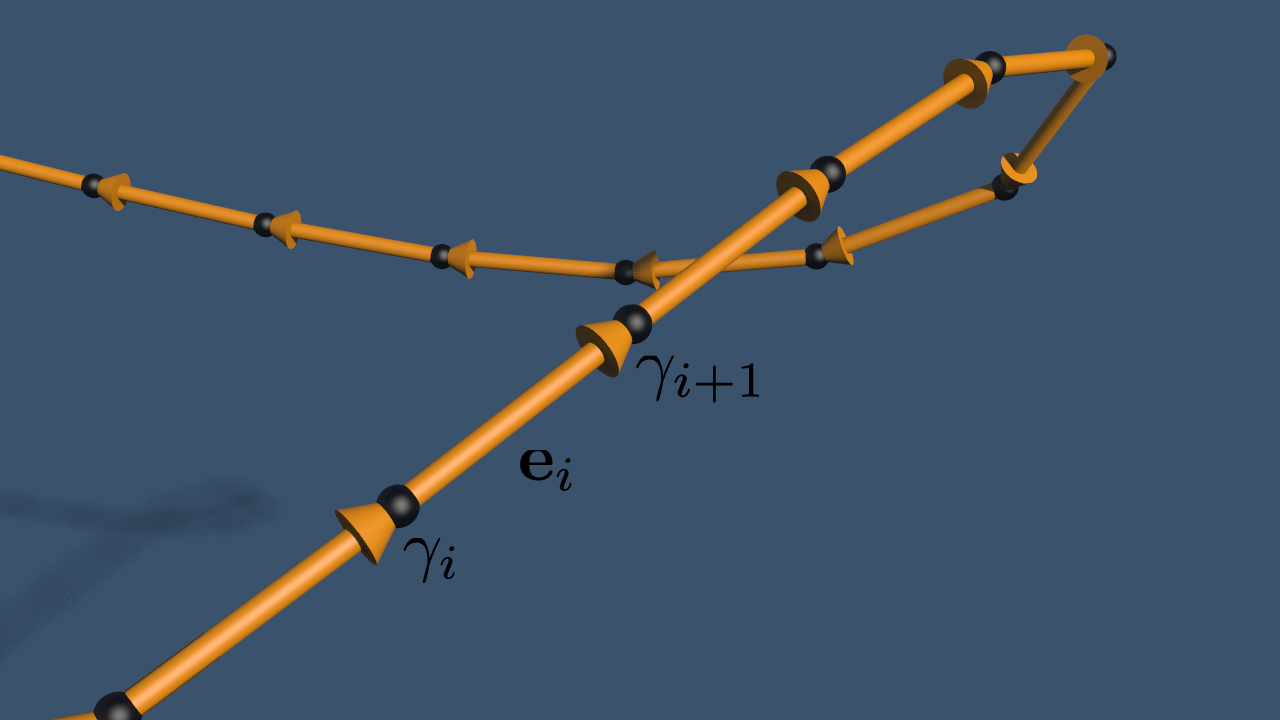
A discrete curve \(\gamma\) in a space \(\mathrm M\) is just a finite sequence of points in \(\mathrm M\), \(\gamma = (\gamma_0,…,\gamma_{n-1})\). In case we have discrete curve \(\gamma\) in \(\mathbb R^3\) we can simply draw \(\gamma\) by joining the points by straight edge segments.

tangents_

The vector that moves a point \(\gamma_i\) to the next point \(\gamma_{i+1}\) is called the discrete tangent vector \[\mathbf e_i := \gamma_{i+1}-\gamma_i.\]Further, the normalized tangent vector will be denoted by\[T_i := \frac{\mathbf e_i}{\Vert\mathbf e_i\Vert}.\]It is even more convenient to draw the points as small spheres and the lines as tubes that align with the corresponding edge. Actually there is 1-parameter freedom to place the tube around the edge – we could rotate the tube around the edge – which is hidden in the tube’s rotational symmetry.

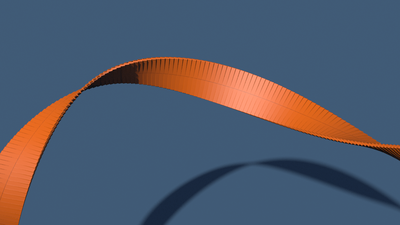
If we instead would like replace the edges by a less symmetric shape (as e.g. in Albert’s post) or if we want to really mesh a tubular surface around the curve this freedom matters. Therefore we must additionally specify a direction in the normal space of the edge.

strip_

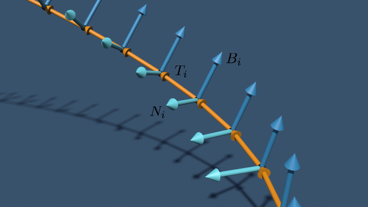
A discrete normal vector field of \(\gamma\) is a sequence \(N= (N_0,…,N_{n-2})\) such that\[N_i\perp T_i, \textit{ for all }i=0,…,n-2.\]For convenience, \(\mathcal N_i:=T_i^\perp\). Given such a discrete normal vector field \(N\) we automatically obtain a second normal vector field from it:\[B := T\times N.\]The triple \(\sigma= (T,N,B)\) then yields at each vertex an oriented orthonormal basis of \(\mathbb R^3\), where the first vector aligns with the tangent direction. This kind of object are well-known in differential geometry and in analogy to the smooth case we will call it a discrete frame.

frame__

Like in the smooth case,  there are distinguished frames among all the possible ones. A quite old-fashioned but still famous notion is the Frenet frame (see e.g. this wikipedia entry). We will instead work with parallel frames here:

The discrete parallel transport is map that assigns to each point \(i\) a rotation \(P_i\in \mathrm{SO}(3)\) that describes how the normal spaces \(\mathcal N_{i-1}\) and \(\mathcal N_i\) are connected: If \(T_{i-1}\times T_i = 0\)  we set \(P_i=\mathrm{id}\), else \(P_i\) is the unique rotation around \(T_{i-1}\times T_i\) that maps \(T_{i-1}\) to \(T_i\), i.e.\[P_i(T_{i-1}) = T_i, \quad P_i(T_{i-1}\times T_i) = T_{i-1}\times T_i.\]Now, let \(N\) be a discrete normal vector field of the discrete curve \(\gamma\). We say \(N\) is parallel, if \[N_i = P_i(N_{i-1}), \quad i =1,…,n-2.\]A parallel discrete frame is then a discrete frame \((T,N,B)\), where \(N\) (and consequently \(B\)) is a parallel discrete normal vector field.

In Houdini rotations are stored as quaternions. So it is convenient to describe the parallel transport in quaternions, i.e. we want to find \(q_i\in \mathbb H\), \(\Vert q_i\Vert=1\) such that \[P_i(X)= q_i\,X\,\overline{ q_i}, \quad X \in \mathcal N_{i-1}.\]Here we identified \(\mathbb R^3\) with the imaginary quaternions (compare with Albert’s post):\[\mathbb R^3 \ni (x,y,y) \longleftrightarrow x\,\mathbf i + y\,\mathbf j + z\,\mathbf k \in\mathrm{Im}(\mathbb H).\]Now let us find a formula for \(q_i\). First, recall that if \(\mathbf v\in \mathbb R^3\), \(\Vert \mathbf v\Vert=1\), then the rotation around \(\mathbf v\) by the angle \(\alpha \in\mathbb R\) is given by the quaternion\[\cos\bigl(\frac{\alpha}{2}\bigr) + \sin\bigl(\frac{\alpha}{2}\bigr)\mathbf v .\]

The first condition on \(P_i\) tell us that \(q_i = a_i + \mathbf v_i\) where \(\mathbf v_i \perp T_{i-1},T_i\). In particular, \(T_{i-1}\overline{q}_i = q_i\, T_{i-1}\). The second condition then yields that \[T_i = q_i\, T_{i-1}\, \overline{q}_i =q_i^2\, T_{i-1}\]and hence\[\bigl(a_i^2 – \Vert\mathbf v_i\Vert^2\bigr) +2a_i \mathbf v_i = q_i^2 = -T_i T_{i-1} = \langle T_i,T_{i-1}\rangle – \mathrm{Im}\bigl(T_iT_{i-1}\bigr).\]Here we used that \(T_{i-1}^{-1}= -T_{i-1}\). Further, since \(\Vert q_i\Vert =1\), we obtain \(1 – a_i^2=  \Vert \mathbf v_i\Vert\), which we can substitute into the equation above. Comparing real and imaginary part then yields two equations\[a_i^2 =\frac{1+\langle T_i,T_{i-1}\rangle}{2}, \quad \mathbf v_i = -\frac{1}{2a_i}\mathrm{Im}\bigl(T_iT_{i-1}\bigr).\]

Note that the equation above determines \(q_i\) only up to sign. Therefore we can assume that \(a_i\geq 0\). Hence we end up with the following formula for \(a_i\) and \(\mathbf v_i\):\[a_i = \sqrt{\frac{1+\langle T_i,T_{i-1}\rangle}{2}},\quad \mathbf v_i = \frac{-1}{\sqrt{2+2\langle T_i,T_{i-1}\rangle}}\mathrm{Im}\bigl(T_iT_{i-1}\bigr).\]

Now given the discrete parallel transports we can easily construct a parallel normal field \(N\) as follows: Choose some vector \(N_0\) normal to the first edge. Then propagate this vector to the whole curve using the transport,\[N_i := P_i\circ\cdots\circ P_1(N_0) = \underbrace{q_i\cdots q_1}_{=:\mathfrak q_{0,i}} \,N_0\, \overline{q}_1\cdots \overline{q}_i =\mathfrak q_{0,i}\, N_0 \, \overline{\mathfrak q_{0,i}}.\]

Actually that is what is used by Albert to orient the chain links: The chain link is a fixed geometry in its own coordinate system. The copy node makes for each point a copy which is then translated to the current point’s position and stretched by the attribute @pscale. If the node finds an attribute named @orient (a quaternion store as vector4), it additionally performs the corresponding rotation. Hence if the chain was aligned with the \(x\)-axis (i.e. with the quaternion \(\mathbf i\)) we need to specify quaternions that rotate the vector \(\mathbf i\) to the corresponding tangent vectors \(T\). Therefore we can choose any quaternion, say \(\psi_0\), to get the rotation from \(\mathbf i\) to the first edge \(T_0\),\[T_0 = \psi_o\mathbf i\,\overline{\psi_o},\]before we use the parallel transports \(q_i\) to get the other rotations:\[\psi_i := q_i\cdots q_1\psi_0.\]

Homework (due 10/12 May): Rebuild the chain rendering presented in the previous post. Write two networks: one using the closed arclength-parametrized curves from Ulrich’s post, and a second one that uses the curve node to build up a generic closed curve as input. (Use the resample node to make it arclength-parametrized).

Posted in Tutorial | Comments Off on Tutorial 2: Framed Discrete Curves

Mandelbrot Set

If you google “mathematics visualization”, the resulting wikipedia page shows the Mandelbrot set as a famous example.

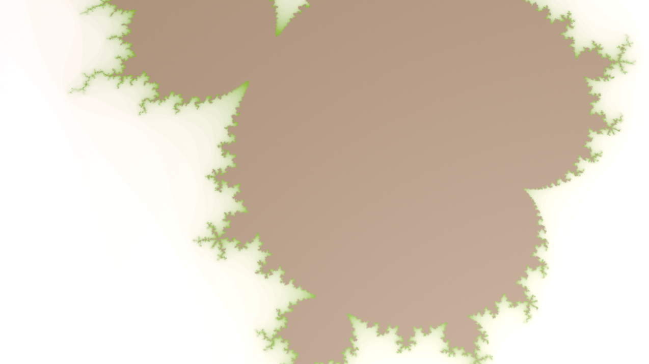
The Mandelbrot set \(M\subset{\Bbb C}\) is defined as the following.  For each \(c\in {\Bbb C}\), consider the iteration \(z_{n+1}(c) = ({z_n}(c))^2+c\), \(n=0,1,2,\ldots\) and \(z_0(c) = 0\). Observe that if \(|c|\) is small, say 0.1, then this iteration yields a sequence \(z_n(c)\) that remains bounded as \(n\rightarrow \infty\).  If \(|c|\) is large, say greater than 2, then \(|z_n(c)|\rightarrow \infty\) as \(n\rightarrow \infty\).  The Mandelbrot set \(M\) is the set of \(c\) which results in a bounded sequence \(z_n(c)\).

Most visualizations of Mandelbrot set you could find on web are colorful images on \({\Bbb C}\).  The color at \(c\) usually indicates the number of iterations it takes before \(|z_n(c)|\) exceeds 2 (which implies \(c\) must not be in \(M\)).  More precisely, people plot the function \(k:{\Bbb C}\rightarrow {\Bbb N}\cup\{0\}\)

\[k(c):=
\begin{cases}
0,& c\in \overline M\\
\min\big\{n\,\big|\, |z_{n}|>2\big\},& c\neq \overline M.
\end{cases}
\]

The algorithm for generating such \(k\) is straightforward.

  1. Put a grid of points \(\{c_j\}\subset {\Bbb C}\) (the points on which you want to evaluate \(k\)).
  2. Initialize \(k_j = 0\). (This \(k_j\) means \(k(c_j)\)).  Initialize \(z_j = 0\).  Initialize iteration number \(n=0\).
  3. Now repeat the following
    1. Replace \(n\) by \(n+1\);
    2. For each point \(j\), if \(k_j=0\), then
      1. replace \(z_j\) by \(z_j^2+c_j\),
      2. if \(|z_j|>2\) then set \(k_j=n\).

Implementing Mandelbrot set in Houdini would be a good exercise for

  • creating point attributes representing complex numbers.
  • iterations.
  • writing functions which implements squaring complex numbers.

Step 1. Create a grid and assign point attributes

In /obj/ network port create a Geometry.  Dive in this geo1, delete the default file1 node, and create a Grid.  Choose its orientation “ZX Plane” with size 3\(\times\)3 centered at \((0,0,-0.5)\).  Set Rows and Columns 100\(\times\) 100.  After everything works, you may increase rows and columns.

Create a PointWrangle node downstream of grid1.  Make sure the option “Run Over” is “Points”.  Write code

Here we created 3 point attributes: @z, @c and @k. Variables with prefix @ indicates that it is really some data defined on, in this case, each point. These variables would be pass to next node downstream; on the contrary variables without the prefix @ are local variables. For instance @P is the point position (of type “vector”) that has been defined. To define new attribute named name, write f@name for float data type, i@name for int data type, v@name for vector data type… See “Accessing Geometry Attributes” in the following page
http://www.sidefx.com/docs/houdini15.0/vex/snippets#attributes

In particular, the “vector2” data type is a natural choice for complex numbers. For a variable A of type “vector2”, its component is accessed as “A.x and A.y“, or equivalently “A.u and A.v“.

If you have a 3-button mouse with middle click as an ordinary middle click, long press your middle button on this PointWrangle node to observe the newly created attributes.

Step 2. Build an iteration

There are a few ways to run iterations in Houdini.  One way is to use “ForLoop” node.  Another way is to turn the “time line” of Houdini into our iteration.  We will use the latter approach.

Create a Solver node downstream of the above PointWrangle node. Dive into this solver node. You will observe a (purple) node labeled “Previous Frame”. As one plays animation, this “Previous Frame” node takes data of the “rendered” node of the previous time frame, which allows us to implement iteration.

One also sees that the path of this solver node is quite complicated: /obj/geo1/solver1/d/s. Recall that in /obj there are only limited nodes one could create; that is the land of objects where one creates geometry node or camera or lights. In /obj/geo1 one can create all “SOP nodes” (the nodes we would be working mostly); this is a SOP land or (the land of geometry). You could take a look at /obj/geo1/solver1, it is also a land of SOP. But in /obj/geo1/solver1/d, it is a “DOP land”, the land of dynamics. The nodes you could create in a DOP land is very different from that in SOP land. It contains drivers that are related to the Houdini time line. There is a particular DOP node called “SOP solver” which is a subnetwork in which one has again an SOP land. Before you learn how to take control of DOP network, you don’t need to know any of these details. This solver node already build the DOP part for you, and all you need is to work in /obj/geo1/solver1/d/s, which is an SOP land.

Here is an important trick. Go to /obj/geo1/solver1/d, and on the parameter board, uncheck “Solve Objects on Creation Frame”. If it is checked, then at Frame 1 it would show the result already after one iteration; we uncheck it because usually we want to look at the initial state at Frame 1.

Let us return to /obj/geo1/solver1/d/s. Create a PointWrangle node. This is where we implement the algorithm for Mandelbrot set. Recall that in the algorithm, we need the iterator \(n\). In our case \(n\) is the frame number. We would like to access Houdini’s frame number. Here is a robust way of doing so:

  • On the top-right of the parameter panel of this PointWrangle node, you can see a “gear” icon; click on it and choose “Edit parameter interface…”.
  • You should see a window with 3 columns.  On the left (Create Parameter) find the item “Integer”.  Drag the “Integer” to the middle column (Existing Parameter) and insert it right above the Code folder.
  • The right column (Parameter Description) shows the property of this newly created UI.  Change the “Name” to n, and change the label to whatever you want (I’ll make it n as well).  Click Apply or Accept and close the window.  You should see a new slider of integer is created.  When your mouse curser runs over its label, you should see “Parameter: n“.
  • Now, in the box for entering values of n, type $F. This is the global variable of time frame which can be called from these value boxes.

Now we can write code in the VEX expression box.

If you happen to copy this code, make sure you have the “>” symbol fixed (WordPress doesn’t let me type the ordinary “>” symbol).

Note that every time I refer to the data @z, I explicitly write it with prefix u@z to keep declaring it is a vector2 variable. Sometimes Houdini just forgets the type of attributes and treat them as floats, creating some hard-to-find bugs. (Likewise one could also replace @k with i@k).

Finally, make this PointWrangle node rendered (turn the blue light on).

Step 3. Visualize the function k

Go back to /obj/geo1 and create another PointWrangle node downstream of the solver node. Click the gear icon \(\rightarrow\) edit parameter interface…, drag and drop a “Ramp (color)” parameter into the existing parameter column (right above the code folder). Name it “colorbar”.  Accept and go back to the wrangle node.  You can design your own colorbar using this UI.

In the VEX expression, type

Finally, if no error has been made, play animation. One should obtain a visualization of the Mandelbrot set:

Screen Shot 2016-04-27 at 12.20.31 AM

Additional fun visualization

You may find that some part of the Mandelbrot fractal looks similar to the terrain of mountains and creeks.  How about really creating such terrain in Houdini?

Go back into the Solver node.  Create a “Soft Transform” node. In the “Group” box, type @k=$F. In the “translate” y-channel, type -0.2/$F. In the “Soft Radius”, type 1/$F.

Screen Shot 2016-04-27 at 12.58.00 AM

Posted in Tutorial | Comments Off on Mandelbrot Set

Conformal Maps I: Holomorphic Functions

If $M\subset\mathbb{R}^2$ is a plane domain and the image of parametrized surface $f:M\to \mathbb{R}^3$ is contained in

\[\mathbb{R}^2=\{(x,y,z)\in \mathbb{R}^3\,\,|\,\, z=0\}\]

then the defining equations of a conformal map

\begin{align*}\left|f_u\right|&=\left|f_v\right| \\\\ \langle f_u,f_v\rangle &=0\end{align*}

imply that $\left|f_v\right|$ arises from $\left|f_v\right|$ by a $90^\circ$-rotation, either counter-clockwise,

\[f_v=J\,f_u\]

or clockwise:

\[f_v=-J\,f_u.\]

Here

\[J = \left(\begin{array}{cc}0 & -1 \\ 1 & 0\end{array}\right)\]

is the matrix corresponding to the $90^\circ$-rotation in the positive sense. Let us stick to the first possibility $\left|f_v\right|=J\left|f_u\right|$ which corresponds to the case where the map $f$ preserves orientation. If you spell out what this property means for the two component functions of $f$, you will find this relation to be equivalent to the Cauchy-Riemann equations. So, if we identify $\mathbb{R}^2$ with the set $\mathbb{C}$ of complex numbers, orientation-preserving conformal maps from domains in $\mathbb{R}^2$ into $\mathbb{R}^2$ are holomorphic maps. Note that the above matrix $J$ has the same effect on vectors in $\mathbb{R}^2=\mathbb{C}$ as multiplication by $i$.

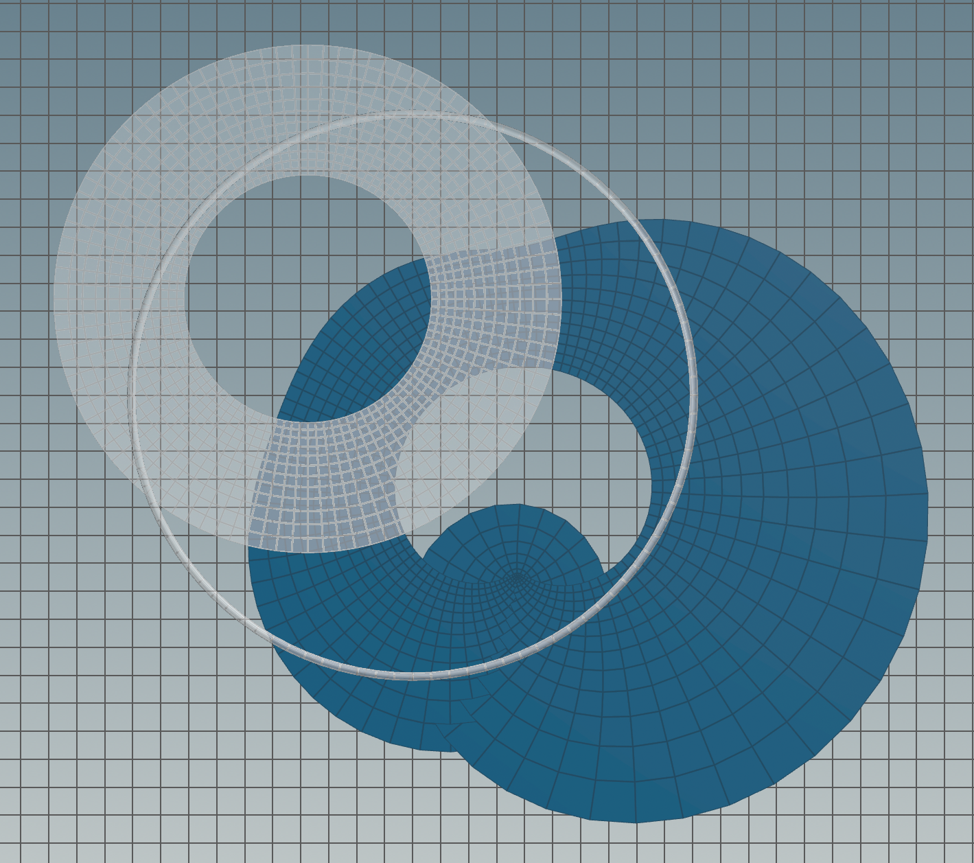
The above observation supplies us with a rich source for conformal parametrizations. At least away from the zeros of their derivative, all holomorphic maps are conformal. For example, all complex polynomials are conformal. Below we show the map

\begin{align}f: M &\to \mathbb{C} \\ f(z) &= \frac{z^4}{4}-z\end{align}

where $M$ is a certain annulus (shown in white). To help orientation in $\mathbb{C}$, we also displayed the unit circle. Not that the roughly square-shaped quadrilaterals of the annulus approximately retain their shape, basically they are only scaled.

holomorphic

Posted in Lecture | Comments Off on Conformal Maps I: Holomorphic Functions

Conformal Parametrizations of Surfaces

In the context of surfaces the strict analog of arclength parametrized curves is an isometric immersion

\[f: M\to \mathbb{R}^3\]

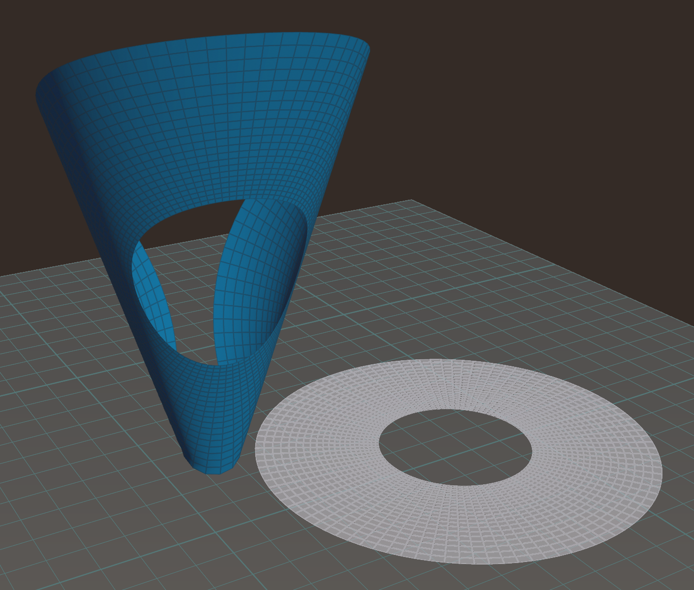
of a standard surface into $\mathbb{R}^3$. Here “isometric” means that lengths of curves and intersection angles of curves on the surface remain the same as they were on the standard surface $M$. As an example, here is an isometric immersion of an annulus in $\mathbb{R}^2$:

isometric-2

Here we used in a Point Wrangle node the following VEX code that wraps the $z,x$-plane isometrically around a cone:

If the parameter domain is a subset $M\subset \mathbb{R}^2$, the standard coordinates of $\mathbb{R}^2$ are labeled $u,v$ and subscripts denote partial derivatives then $f$ is isometric if and only if

\begin{align*}\left|f_u\right|=\left|f_v\right|&=1 \\\\ \langle f_u,f_v\rangle &=0.\end{align*}

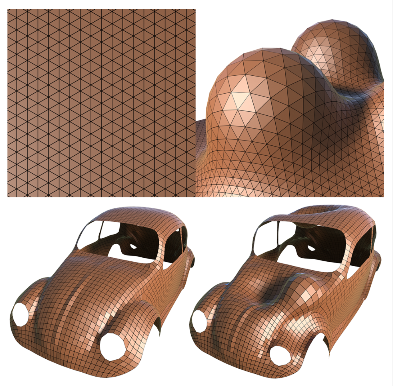
Very few surfaces admit such an isometric parametrizations. Also the possible isometric deformations of a given surface in $\mathbb{R}^3$ are quite limited and rigid. We therefore look at the larger class of conformal deformations, which preserve intersection angles of curves on the surface but not the length. So local features are enlarged or shrunk but not distorted.

conformal

A parametrization $f$ defined on a domain $M\subset \mathbb{R}^2$ is conformal if and only if the exists local scalings  $e^\phi$ defined by a function $\phi: M \to \mathbb{R}$ such that

\begin{align*}\left|f_u\right|=\left|f_v\right|&=e^\phi \\\\ \langle f_u,f_v\rangle &=0.\end{align*}

For many applications (including numerical computations) it is desirable that the triangles of a simplicial surface are as equilateral as possible. Similarly often the quadrilaterals of a quadrilateral mesh should preferably as square-shaped as possible. Conformal deformations have the pleasant feature that they do not deteriorate the quality of the mesh (when measured in this sense).

Posted in Lecture | Comments Off on Conformal Parametrizations of Surfaces

Parallel Frame for Curves

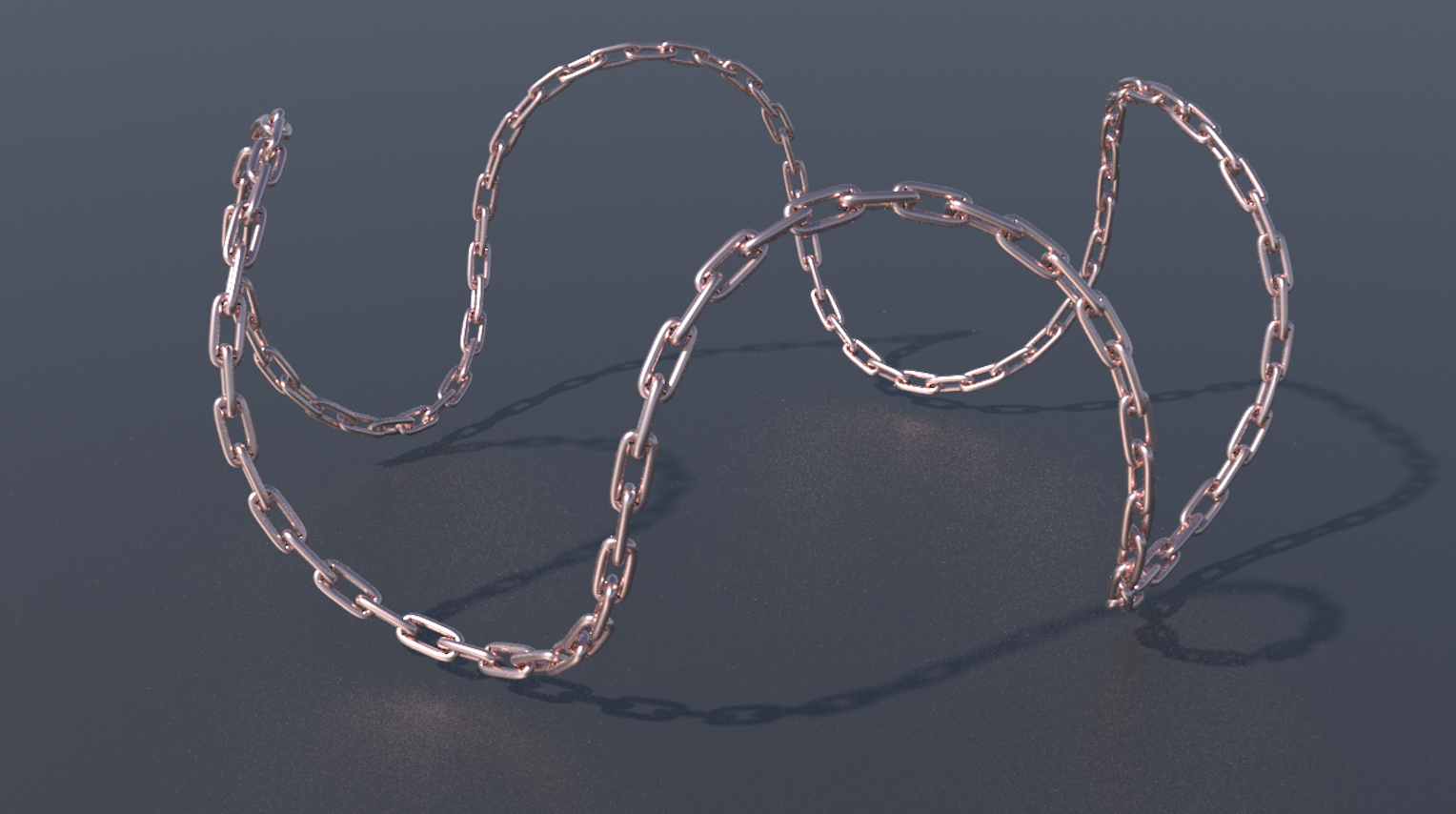
If you have a polygonal curve, say arc-length parameterized, you might want to visualize the curve as the following rendering

curve

This can be done in Houdini by the “copy” SOP node.

The “copy” node has two input and one output.  The first input (left input) takes a geometry that is to be copied, for instance one metal ring of the linked chain; the second input (right input) is a set of points at which the copied geometries would locate, for example the polygonal curve.

A small trick for using the “copy” node: in the copy node, go to the “Stamp” tag, and turn on “Pack geometry before copying”.  It would be much more efficient and memory saving.

If you connect a piece of geometry (like the ring for the chain) to the first input of “copy” and a curve to the second input of “copy”, you would see that the rings are indeed copied and translated to the vertices of the curve.  But they are not oriented as the above figure.  The “copy” node creates copies of the first input and is able to transform (translate, rotate and scale) the copied geometry by reading the point attributes of the second input.  For example it reads the point attribute @P (of type vector) to translate the copied geometry.  To control the orientation of the copied geometry, the copy node reads the attribute @orient (of type vector4, i.e. quaternions). Since the attribute @orient  has not been setup on points, it only has default orientation.

A complete list of point attributes the copy node would read can be found here
http://www.sidefx.com/docs/houdini15.0/copy/instanceattrs

Quaternions

Quaternions can represent 3D orientation (3D rotation).  Quaternion \({\Bbb H}\) is a number system like complex number but with 3 imaginary dimensions; together with the real part, a quaternion is a 4-vector:

\[q\in{\Bbb H},\quad q = w+x{\bf i}+y{\bf j}+z{\bf k}\]

with multiplication rules:

\[{\bf i}^2 = {\bf j}^2 = {\bf k}^2 = -1,\quad {\bf ij}=-{\bf ji}={\bf k}, {\bf jk}=-{\bf kj}={\bf i}, {\bf ki}=-{\bf ik}={\bf j}.\]

For each 3D vector \({\bf v} = (v_x,v_y,v_z)\) one can view it as a purly imaginary quaternion \({\bf v} = v_x{\bf i}+v_y{\bf j}+v_z{\bf k}\).  Then

\[q{\bf v}q^{-1}\]

is again a purely imaginary quaternion, and as a 3D vector, it is a rotation of \({\bf v}\). (Here \(q^{-1} = \overline q/|q|^2\), just like complex numbers).  Quaternionic rotations are very useful because they describe rotations by “angles” and “axis to rotate about”.  If you want to rotate \(\theta\) angle about an axis \({\bf a}\) (a 3D vector with \(|{\bf a}|=1\)), then the corresponding quaternion is given by

\[q = \cos\left({\theta\over 2}\right) + \sin\left({\theta\over 2}\right){\bf a}.\]

In addition, if you would like to rotate something by \(q_1\) and then by \(q_2\), the resulting rotation is simply \(q_2q_1\). This is because quaternion multiplications are associative
\[(q_2q_1){\bf v}(q_2q_1)^{-1} = q_2(q_1{\bf v}q_1^{-1})q_2^{-1}.\]
Note that quaternion multiplications are not commutative, i.e. \(q_1q_2\neq q_2q_1\) in general.

In Houdini’s VEX language, quaternions are of vector4 type. To access the components of a vector4 variable, use w (real part) and x,y,z (imaginary) fields. For example

Fortunately, you can simplify the above code using Houdini’s VEX function vector4 quaternion(float angle, vector axis):

In Houdini, if you want to multiply two quaternions q1, q2, use

vector4 Q = qmultiply(q1,q2);

Parallel Frame

Now we know how to represent orientation in Houdini.  We could define p@orient (p@ declares a vector4; equivalently, you may define it by vector4 @orient;) in a PointWrangle node for the curve before it enters the copy node.

But how should we orient these points on curve so that it looks most natural? Look carefully at the above rendering. Imagine each prolonged ring is a tangent vector of the curve, then two adjacent tangents form a plane (called osculating plane). Notice that two adjacent rings are just differ by a rotated within this osculating plane (rotation about the normal of osculating plane) (ignoring the \(\pi\over 2\) rotation about the tangent vector which is just for rings to interlocked). Such orientation field on a curve is called a parallel frame, i.e., there is no twist of the frame along the curve. (Chain of interlocked rings does not admit twists.)

Suppose there are \(n\) points in this polygonal curve with position \(P_0,\ldots,P_{n-1}\in{\tt vector}\). We can assign a tangent vector to each point \(T_j = {\tt normalize}(P_{j+1}-P_j)\). We would like to assign the point attribute @orient as \(Q_0,\ldots,Q_{n-1}\in{\tt vector4}\) recursively with
\[Q_{j+1} = q_jQ_j\]
where
\[q_j = {\tt quaternion}(\theta_j,{\tt axis}_j)\]
\[\theta_j = \arccos(T_j\cdot T_{j+1}),\quad{\tt axis}_j = {\tt normalize}(T_j\times T_{j+1}).\]
For the initial \(Q_0\) one could just pick any orientation; a natural choice would be
\[Q_0 = {\tt quaternion}\Big(\arccos(\{1,0,0\}\cdot T_0),{\tt normalize}(\{1,0,0\}\times T_0)\Big),\]
so that it makes sure the \(x\)-axis is always rotated to the tangent vector when using the copy node.

Sample code

After the nodes creating the curve geometry, create a PointWrangle node which we name it “compute_tangent”, and then a AttributeWrangle node which we name it “compute_parallel_frame”.  In the “compute_tangent” node, make sure it “runs over points”.  In the “compute_parallel_frame” node, make sure it “run over details (only once)”.

Compute_tangent:

Compute_parallel_frame:

You may find that I used many functions related to “hedge” (half-edge). Look them up in Houdini’s VEX function reference. It is very useful as an iterator in polygons.

Posted in Tutorial | Comments Off on Parallel Frame for Curves

Arclength-Parametrized Curves

A parametrized curve $\gamma_[0,L]\to\mathbb{R}^3$ is called parametrized by arclength provided that $\gamma(t)$ moves with unit speed if we interpret $t$ as time:

$\left|\gamma'(t)\right|=1$  for all  $t\in [0,L]$.

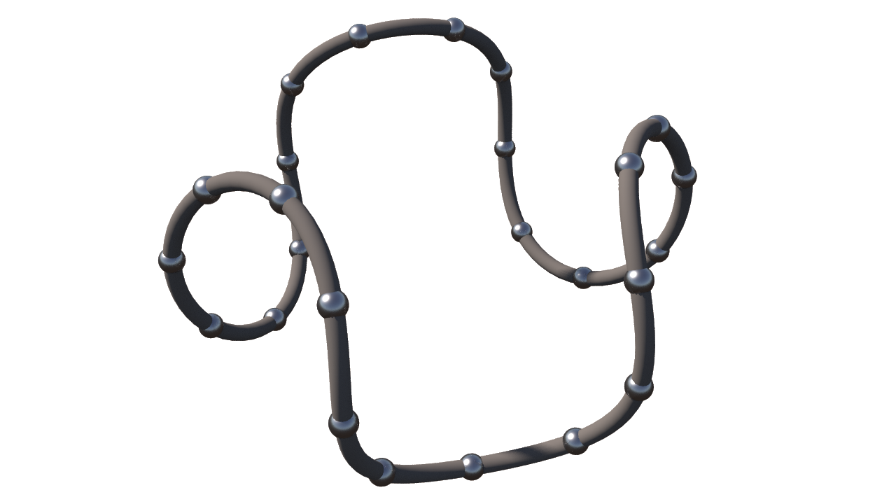
Sampling an arclength-parametrization $\gamma$ at evenly spaced points $t=\frac{mL}{n}$ for integer values of $m$ leads to a division of the curve into $n$ arcs of length $\frac{L}{n}$:

arclength-closed-2

The arclength-parametrized curve above was computed using the explicit formula

\[\gamma(t)=\frac{1}{r+r^{2k-1}}\left(\begin{array}{c}r \cos t +\frac{1}{2k-1}r^{2k-1}\cos((2k-1)t) \\ \frac{2r^k}{k}\sin(kt) \\ r\sin t -\frac{1}{2k-1}r^{2k-1}\sin((2k-1)t)\end{array}\right).\]

with $k=3$ and $r=0.977$. In fact this family exhausts all examples known to me of arclength-parametrizations for closed curves that are given in terms of elementary functions. On the other hand, it is a basic fact of Differential Geometry that every curve can be parametrized by arclength. This however involves an integration that most of the time cannot be performed explicitly.

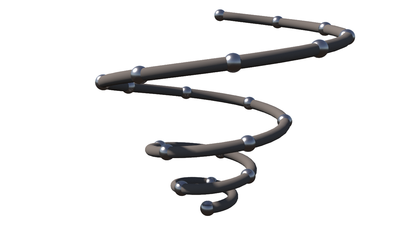
In the discrete world (where curves are polygons with straight edges), parametrization by arclength is easy, because computing the length of any part of the polygon is easy. Houdini provides a node for this purpose called Resample. If we set the parameter Measure of this node to Arc then it will divide the polygon into sub-arcs of equal length:

arclength

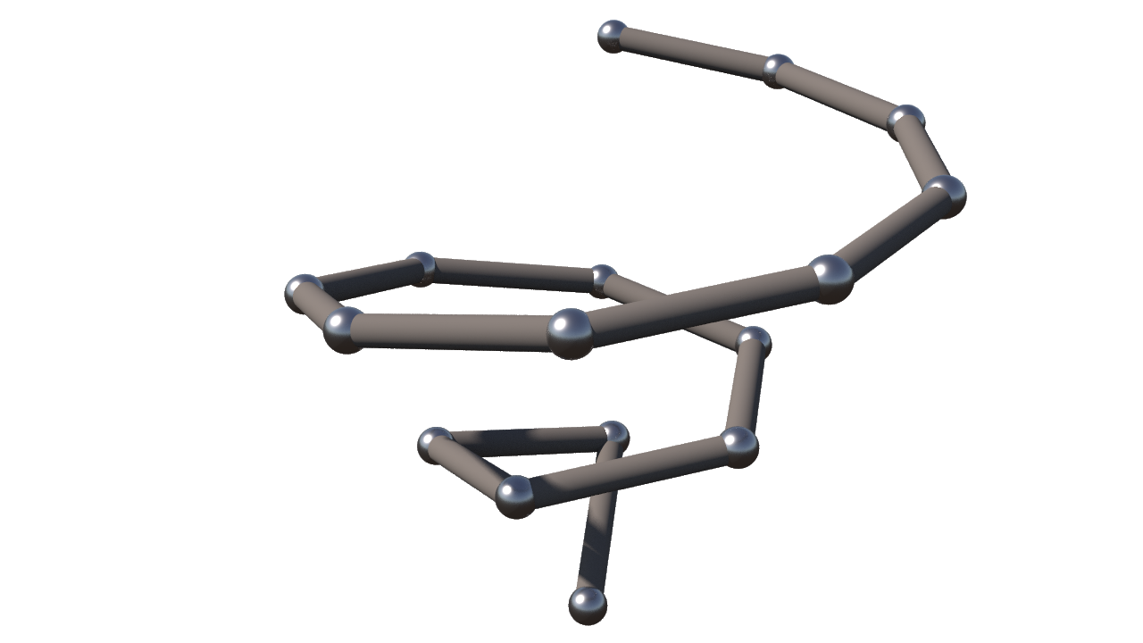
If the goal is instead to sample the curve by a coarser polygon with equal edge length, one can set the Measure parameter to Chord:

cordlength

Posted in Lecture | Comments Off on Arclength-Parametrized Curves

Sampled Parametrized Curves

In the last post we created geometric objects from scratch, including the underlying combinatorics. In most situations it is much more convenient to start with already existing geometry and transform it.

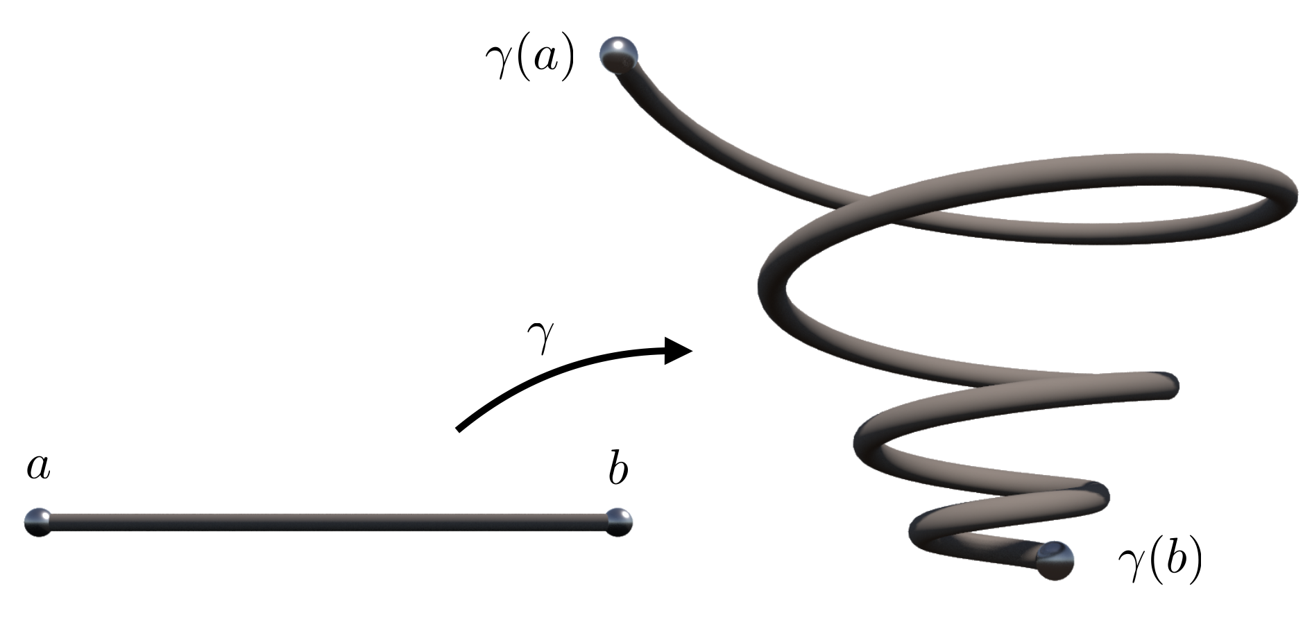
This approach is similar to the standard way of dealing with curves and surfaces in Differential Geometry: One starts with a parameter domain $M$ which could be a subset of $\mathbb{R}^n$ or just an abstract $n$-dimensional manifold. For concreteness, just imagine that $n$ is either one (for the study of curves) or two (for surfaces). The geometric objects of interest are then certain smooth maps $f:M \to \mathbb{R}^3$. Such an $f$ is then called a parametrized curve (in case $n=1$) or a parametrized surface (if $n=2$).

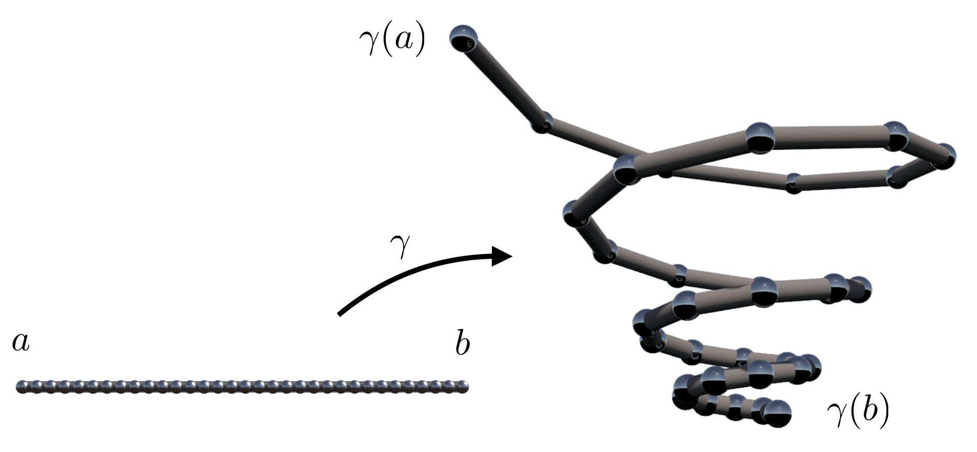
If $M$ is a compact connected one-dimensional manifold with non-empty boundary we can as well assume that $M$ is a closed interval $[a,b]$ on the real line:

curve2

In Houdini a discrete version of the interval $[a,b]$ can conveniently supplied by a Grid node where the Rows has been set to one. The Columns parameter specifies the number of equally spaced sample points on interval. Instead of specifying $a,b$ directly we have to provide $b-a$ as the first component of the Size parameter and $(a+b)/2$ as the first component of the Center parameter. Afterwards we use a node of type Point Wrangle in order to map the $x$-coordinate to the desired space curve. The curve in the last picture results from the VEX code below. alpha, omega and lambda are three float parameters of that Point Wrangle node.

 curve-discrete

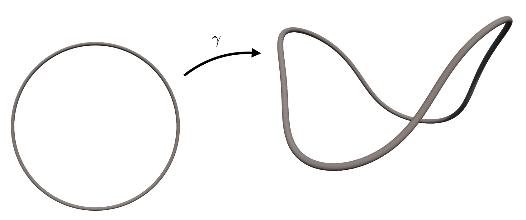
If $M$ is a compact connected one-dimensional manifold without boundary then we can as well assume that $M$ is the unit circle $S^1\subset \mathbb{R}^2$:

closed-parametrized-curve-smooth

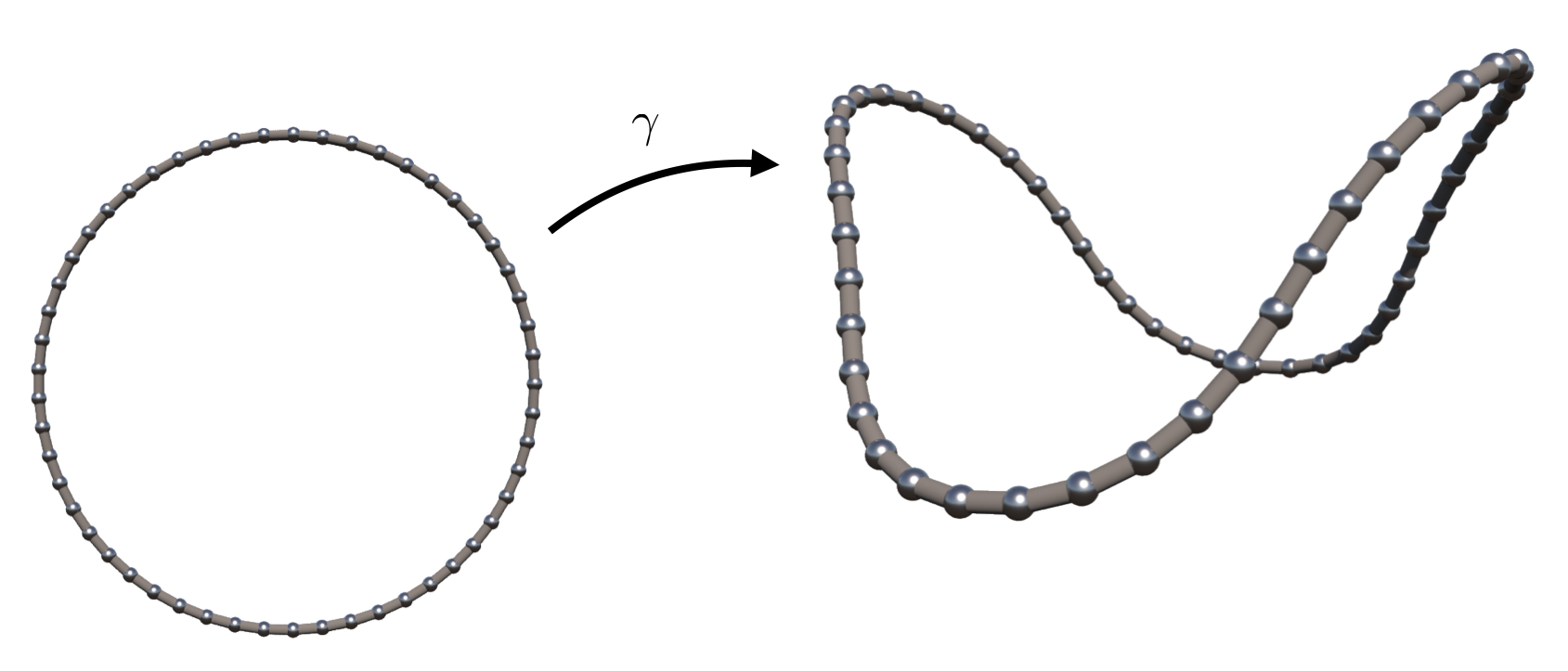
In Houdini a discrete version of the unit circle $S^1$ can conveniently supplied by a Circle node where the Primitive Type has been set to Polygon. The Divisions parameter specifies the number of equally spaced sample points on the circle. Afterwards we use a node of type Point Wrangle in order to map the$(x,y)$-coordinates on the circle to the desired space curve. The curve in the last picture results from the VEX code below. k is an integer parameter and r a float parameter of that Point Wrangle node.

We have used here an include file which implements some complex arithmetic.

closed-parametrized-curve-discrete

Note that the sample points on the space curve roughly look equally spaced. The reason is that in this particular example the corresponding smooth curve is parametrized by arclength for all values of the parameters $k,r$. We leave the proof of this fact as an exercise. This means that if $p$ runs through the unit circle with unit speed then also $\gamma(s)$ travels with unit speed.

Posted in Lecture | Comments Off on Sampled Parametrized Curves

Tutorial 1: Implicit Surfaces with Houdini

It is amazingly simple to create high-quality renderings with Houdini. Several small tricks to achieve nice renderings of geometries in a mathematical context are already described in the first posts of this blog. If you not have looked at it yet you should do it now.

All these posts use standard geometries that come with Houdini. But how do we get other geometries into the scene?

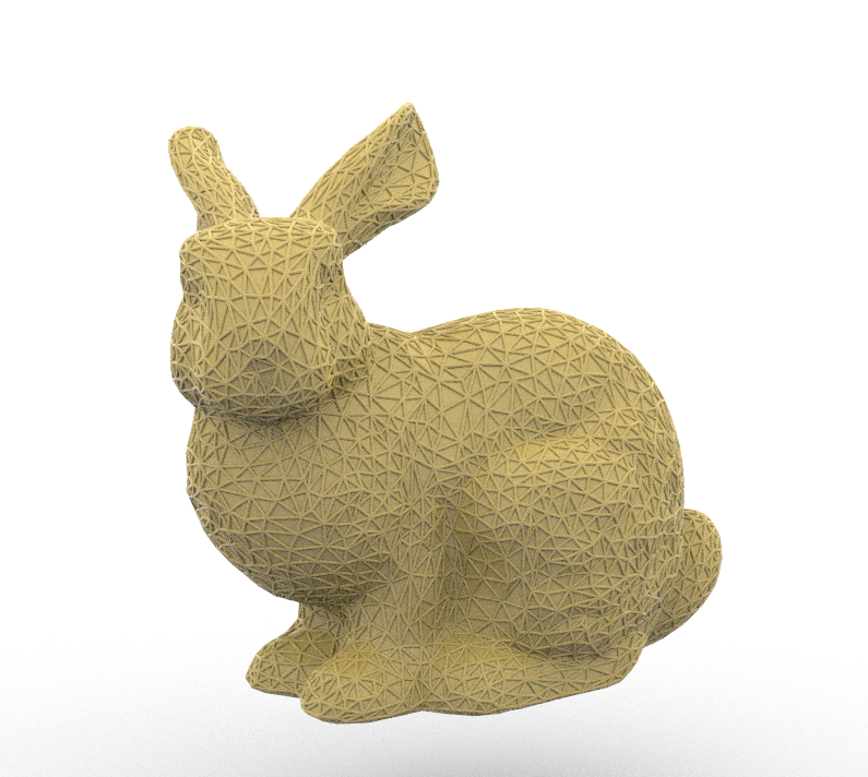
General geometries can be loaded from files (like the Stanford bunny object file). To load the file manually you can use the menu bar: Go to File \(\rightarrow\) Import\(\rightarrow\) Geometry and choose the path of your geometry file. This action creates a geometry node with a file node inside that contains the path. Instead using the menu, one can also use the file node directly. This way we can access geometry files from inside existing networks. A large library of geometry models can be found e.g. at the AIM@SHAPE website.

bunny

Now let us focus on more mathematical surfaces and how to create them using Houdini.

Small geometries can be built up easily using vex code surrounded by an Attribute Wrangle node. A detailed description how this works is given in the post Creating Geometry from Scratch.

Exercise: Play through the examples in “Creating Geometry from Scratch” and additionally build up a network that generates a cube. Choose some materials and colors to create a nice rendering.

Certainly, for larger geometries this way to construct geometries can get arbitrarily complicated and tedious.

A natural source of surfaces in space is the constant rank theorem. For maps between Euclidean space it tells us that if \(f\colon U \to \mathbb R^m\), defined on an open \(U\subset\mathbb R^n\), is a smooth map of constant rank \(k\), then \[\mathrm M = f^{-1}(\{q\}),\quad q\in \mathbb R^m\] is an \((n-k)\)-dimensional submanifold. In particular if \(f\colon \mathbb R^3 \supset U \to \mathbb R\) has full rank, then \(\mathrm M\) is a surface in \(\mathbb R^3\).

Actually Houdini offers a simple node that allows to create such implicit surfaces. It is called IsoSurface. Here one can specify a function in the coordinates \(\$X\), \(\$Y\) and \(\$Z\) on a volume (3D grid)  of a certain size and resolution. Houdini then automatically generates the discrete surface that corresponds to the zero set of the given function.

Since the values in the volume are interpolated from the values at the points, the resolution of the grid has strong influence on the quality of the result. If necessary the extracted discrete surface can be post-processed with a Remesh node to obtain a triangulation.

Exercise: Create a small network that uses the IsoSurface node to generate a triangulation of a round cylinder and a torus of revolution.

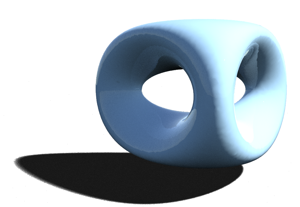
Actually there are implicit formulas to generate surfaces of arbitrary genus. For example, for the so called double-torus, a surface of genus \(2\), a formula can be found on the Wikipedia page on implicit surfaces.

doubletorus

In principle the surfaces and the corresponding functions could become much more complicated. Perhaps one is dealing with a discrete function which is just obtained as a numerical solution of some given problem. In this case an implicit surface can be extracted by the Convert Volume node.

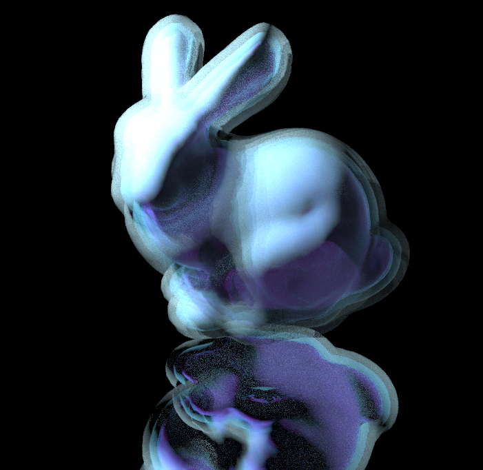
To give some illustration, the function could be e.g. the signed distance function (below the one of the Stanford bunny). From this function we extract the surface itself together with several parallel surfaces: Below a picture of the parallel surfaces – all displayed together using transparency.

parallelbunny

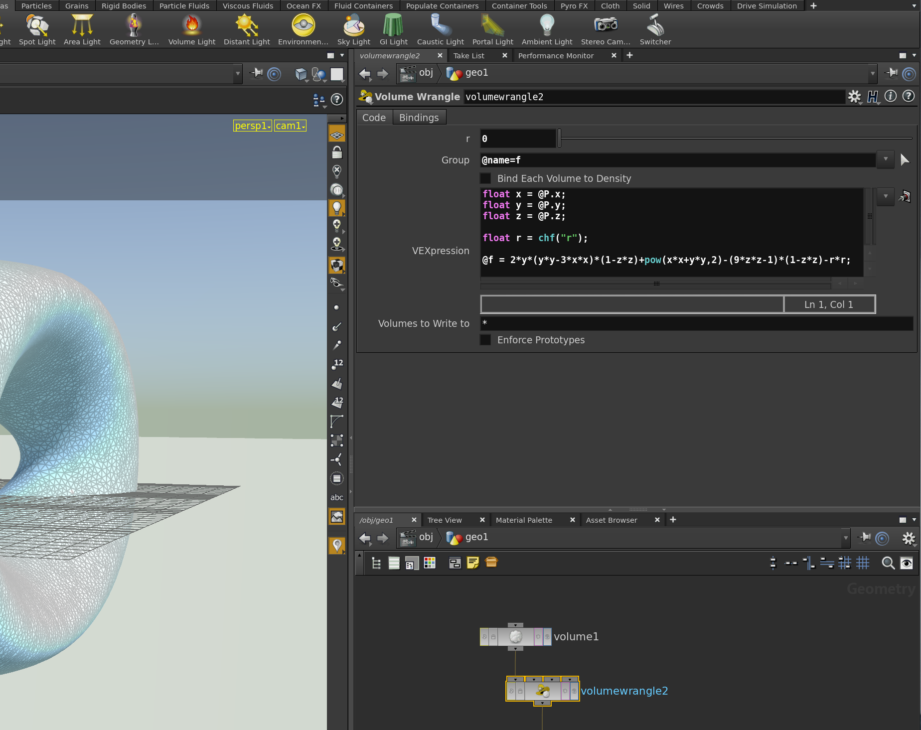
Further, given a Volume (with a specified name), we can use a Volume Wrangle node to write the function values to its points (to set arbitrary boundary values make sure that the border type in the volume properties is set to Streak). In the picture below the volume was named f. One can see how the function values that implicitly define the double torus are written to f using the VEXExpression field of the Volume Wrangle node.

vexExpression

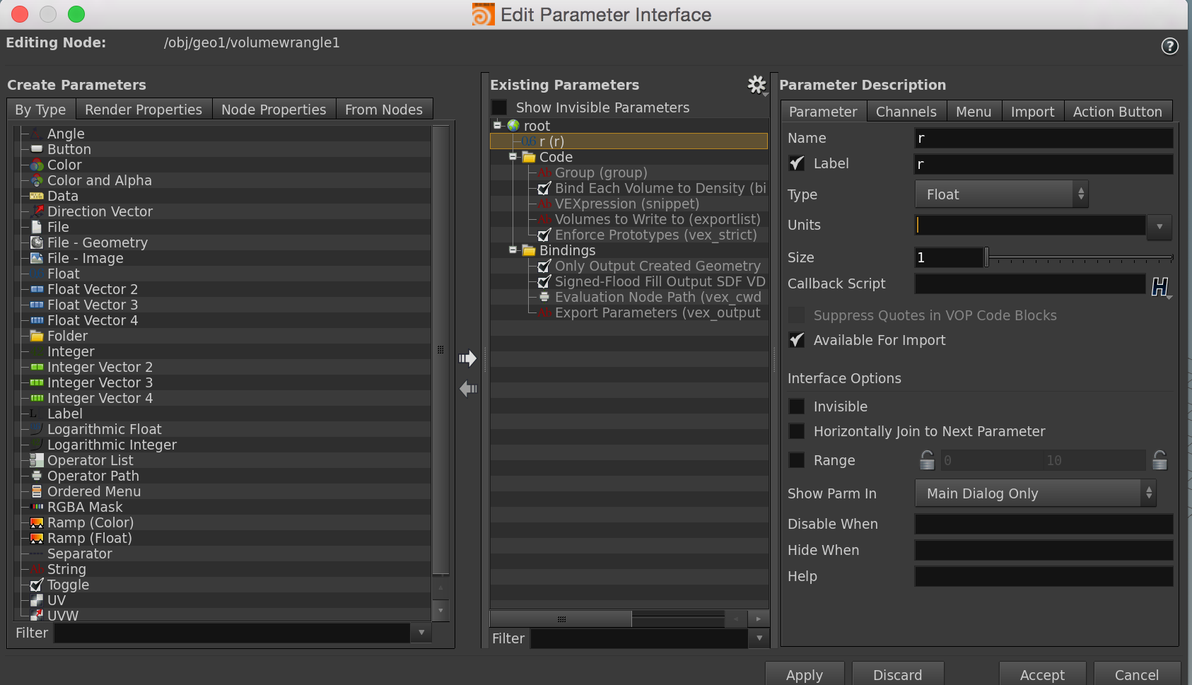
The surface also can be slightly modified by a parameter r, which we added to the node. To do this we can edit the the parameter interface of the node: Right-click on the gear right to the node’s name, choose “Edit parameter interface…”. Then the following panel appears.

parameterinterface

New parameters are created by drag-and-drop: Just pull the Type you need over to the field of existing parameters and give it the name/label/range you want.

Since we can now define our own functions and parameters, this gives us a huge flexibility.

Exercise: Replace the IsoSurface node in the last exercise by a system of 3 nodes – a Volume followed by a Volume Wrangle and a Convert Volume node. Add a float parameter to the parameter interface of the Volume Wrangle which allows to change the radii of the torus.

The Clebsch surface is an algebraic surface in the \(3\)-sphere. Consider the round \(3\)-sphere \[\mathrm S^3 \subset \mathbb R^4 \cong (1,1,1,1,1)^\perp :=\Bigl\{(x_1,…,x_5) \in \mathbb R^5\mid \sum_{i=1}^5 x_i =0\Bigr\} \subset \mathbb R^5.\]The Clebsch surface is then given by the cubic equation\[f(x_1,…,x_5) := \sum_{i=1}^5 x_i^3 =0.\]

clebsch3

The surface lies in the \(3\)-sphere, but we can use the stereographic projection to map it conformally into Euclidean space: If \(\sigma \colon \mathrm S^3\setminus\{\infty\} \to \mathbb R^3\) denotes the stereographic projection, then the image of the Clebsch surface under \(\sigma\) is given by the zero set of the function\[g= f\circ \sigma^{-1}.\]

So let us determine \(\sigma^{-1}\). Usually, if the \(3\)-sphere is considered to lie in \(\mathbb R^4\), the inverse stereographic projection is given by\[\bigl(x_1,x_2,x_3\bigr)\mapsto\frac{1}{\sum_{i=1}^3 x_i^2+1}\Bigl(2x_1,2x_2,2x_3,\sum_{i=1}^3 x_i^2-1\Bigr).\]The only thing that changes here is that we have identified \(\mathbb R^4\) with a hyperplane in \(\mathbb R^5\), so we still need to map \(\mathbb R^4\) isometrically to \((1,1,1,1,1)^\perp\). This amounts to finding an orthonormal basis of \((1,1,1,1,1)^\perp\). So one could for instance the Gram-Schmidt algorithm. But here we can also guess a suitable orthogonal basis: A possible choice is e.g. the following\[\begin{pmatrix} 1 \\ -1 \\ 0 \\ 0 \\ 0 \end{pmatrix}, \begin{pmatrix} 0 \\ 0 \\ 0 \\ -1 \\ 1 \end{pmatrix}, \begin{pmatrix} 1 \\ 1 \\ 0 \\ -1 \\ -1 \end{pmatrix}, \begin{pmatrix} 1 \\ 1 \\ -4 \\ 1 \\ 1 \end{pmatrix}.\]If we normalize these vectors and arrange them into a matrix this yields an isometric immersion \(\mathbb R^4\to (1,1,1,1,1)^\perp\subset \mathbb R^5\). With this we see that \(\sigma^{-1}\) has the following form:\[\sigma^{-1}\bigl(x_1,x_2,x_3\bigr)=\frac{1}{\sum_{i=1}^3 x_i^2+1}\begin{pmatrix} \tfrac{1}{\sqrt{2}} & 0 &\tfrac{1}{2} &\tfrac{1}{2\sqrt{5}} \\ -\tfrac{1}{\sqrt{2}} & 0 &\tfrac{1}{2} &\tfrac{1}{2\sqrt{5}} \\ 0 & 0 & 0 &-\tfrac{2}{\sqrt{5}} \\ 0 & -\tfrac{1}{\sqrt{2}} & -\tfrac{1}{2} &\tfrac{1}{2\sqrt{5}} \\ 0 & \tfrac{1}{\sqrt{2}} &-\tfrac{1}{2} &\tfrac{1}{2\sqrt{5}} \end{pmatrix}\begin{pmatrix}2x_1 \\ 2x_2 \\ 2x_3 \\ \sum_{i=1}^3 x_i^2-1\end{pmatrix}.\]

clebsch

Homework (due 3/5 May): Visualize the Clebsch surface, i.e. write a network that creates a triangulation of the stereographically projected Clebsch surface, choose your favorite materials and colors and render the surface.

Posted in Tutorial | Comments Off on Tutorial 1: Implicit Surfaces with Houdini