Tutorial 3: Framed Closed Curves

A closed discrete curve $\gamma$ is map from a discrete circle ${\mathfrak{S}}_n^1=\{z\in \mathbb{C}\mid z^n=1\}$, $n\in \mathbb{N}$, into some space $\mathrm{M}$. In some situations it is more convenient to consider the discrete circle just as $\mathbb{Z}/n\mathbb{Z}$,$$\mathbb{Z}/n\mathbb{Z}\ni k+n\mathbb{Z}\mapsto e^{2\pi ik/n}\in {\mathfrak{S}}_n^1,$$and a closed discrete curve as a periodic sequence, i.e. $\gamma :\mathbb{Z}\to \mathrm{M}$ such that ${\gamma }_{i+n}={\gamma }_i$. In this case we just write $\gamma =({\gamma }_0,\dots ,{\gamma }_{n-1})$ and keep in mind that it is meant to be a periodic sequence.

Now, if $\gamma =({\gamma }_0,\dots ,{\gamma }_{n-1})$ is a closed discrete curve in ${\mathbb{R}}^3$, we have a corresponding parallel transport $P$. But in general there exists no parallel frame for the curve. This you certainly have noticed already from the last homework.

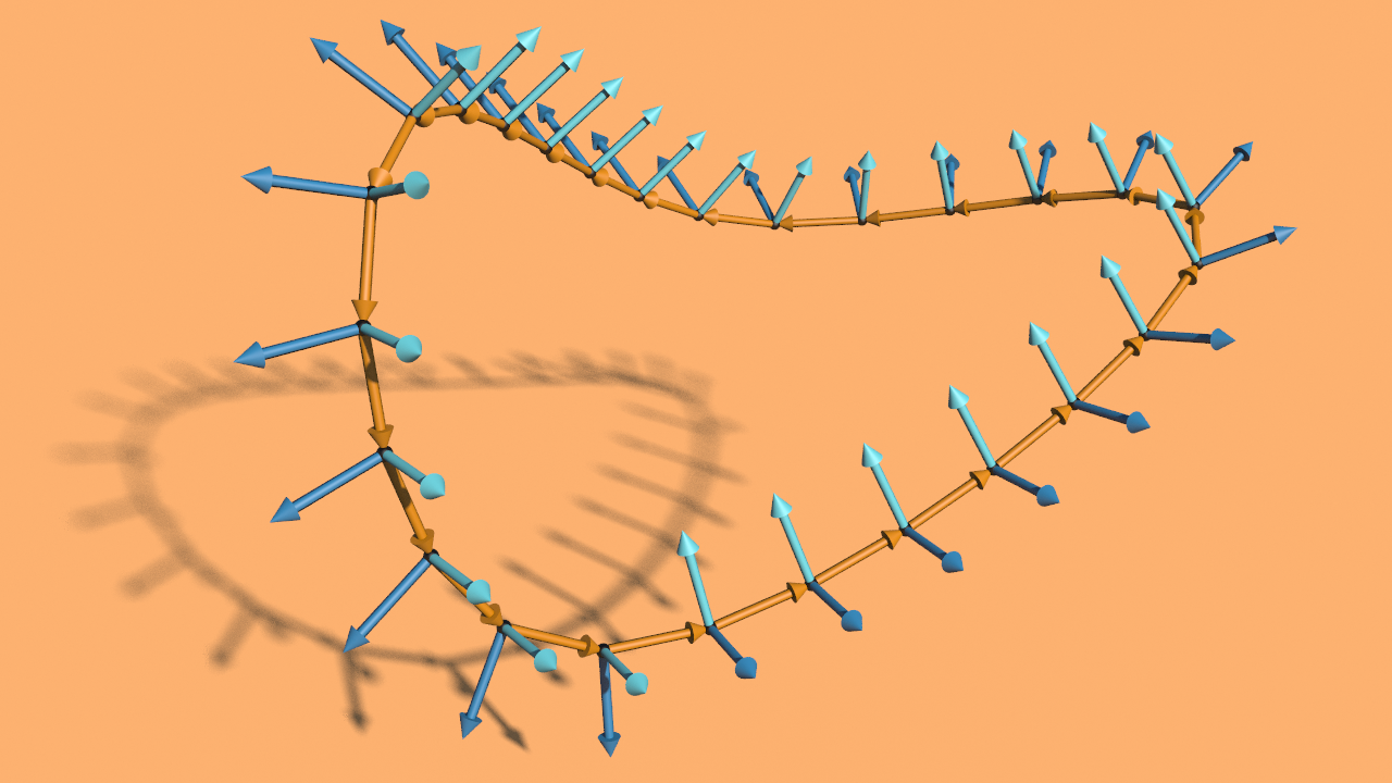
We can still apply the algorithm to the curve and obtain a normal vector field which by construction satisfies $P_k(N_{k-1})=N_k$ for all $k=1,\dots ,n-1$. But there is no reason that this should also be true for $k=n$. Here we may have a certain angle defect $\omega$, $$P_n(N_{n-1})=\cos (\omega )N_0+\sin (\omega )T\times N_0.$$

Note that the normal spaces (and thus also the space of normal vector fields) are natural complex vector spaces. The complex numbers act on ${\mathcal{N}}_k:=T_k^{\perp }$ as follows: $$\mathbb{C}\times {\mathcal{N}}_k\to {\mathcal{N}}_k,(x+iy,N)\mapsto (x+iy)\cdot N:=xN+y{T}_k\times N.$$Further they inherit a natural inner product from ${\mathbb{R}}^3$. This turns the normal spaces into hermitian lines. Note that the parallel transports are isometric orientation preserving maps. Thus they define unitary maps between these lines. For the normal field $N$ defined as above, $$e^{i\omega }{N}_0=P_n(N_{n-1})=P_n\circ \cdots \circ P_1(N_0).$$Hence $$e^{i\omega }=\mathrm{tr}(P_n\circ \cdots \circ P_1).$$ In particular we see that $e^{i\omega }$ is independent of all choices – the choice of the start point $k=0$ and the choice of the first normal vector $N_0$ – and thus can be assigned directly to the curve $\gamma$.

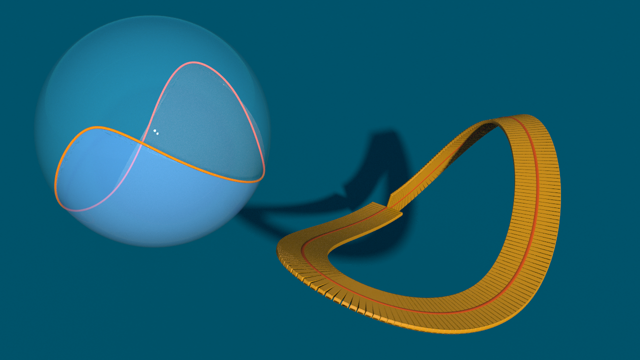
Actually this phenomenon is well-known in the smooth world. The angle defect $\omega$ of a curve $\gamma$ is related to the signed area $A$ enclosed by the tangent $T$ of $\gamma$ on the sphere, $$A\equiv \omega \mathrm{mod}2\pi \mathbb{Z}.$$

Though not each closed discrete curve $\gamma$ can be equipped with a parallel normal field we still want a nice smooth looking framing along the curve. One obvious way to resolve this problem is to distribute the defect $\omega$ along the curve: If $s_k$ denotes the discrete arclength,$$s_k=\sum _{j=0}^{k-1}{\ell }_j,{\ell }_k=\Vert {\mathrm{e}}_k\Vert$$ and $L=s_n=\sum _{j=0}^{n-1}{\ell }_j$ the length of the curve, then the field is given by$${\tilde{N}}_k=e^{-i\frac{\omega }{L}{s}_k}{N}_k.$$Here again $N$ denotes the normal field produced by our algorithm. Note that$$P_k({\tilde{N}}_{k-1})=P_k(e^{-i\frac{\omega }{L}{s}_{k-1}}{N}_{k-1})=e^{-i\frac{\omega }{L}{s}_{k-1}}{P}_k(N_{k-1})=e^{-i\frac{\omega }{L}{s}_{k-1}}{N}_k=e^{i\frac{\omega }{L}{\ell }_k}{\tilde{N}}_k$$for $k=0,\dots ,n-1$. Similarly, for $k=n$ we get$$P_n({\tilde{N}}_{n-1})=e^{-i\frac{\omega }{L}{s}_{n-1}}{P}_n(N_{n-1})=e^{i\omega -i\frac{\omega }{L}{s}_{n-1}}{N}_0=e^{i\frac{\omega }{L}{\ell }_{n-1}}{\tilde{N}}_0.$$I.e. compared to a parallel field the field $\tilde{N}$ rotates by an angle proportional to the edge length.

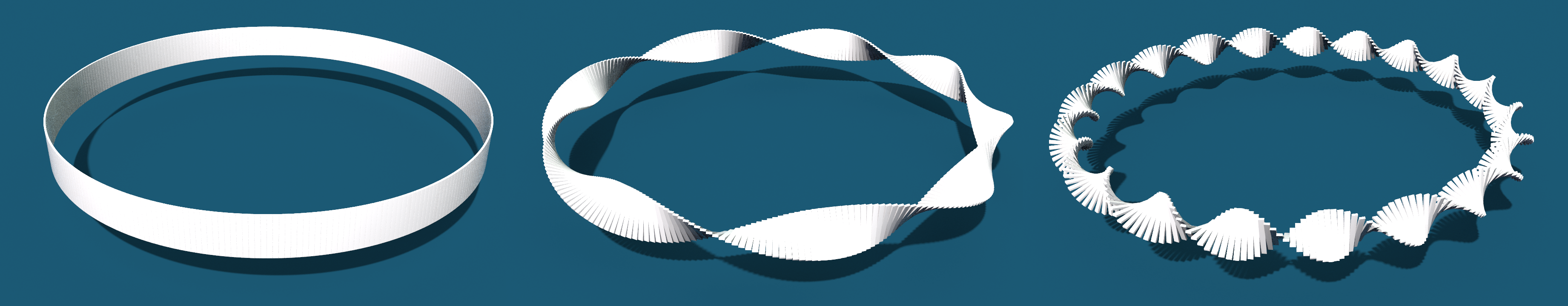
Note that $\omega$ is only defined up to an integral multiple of $2\pi$. The choice of $\omega$ determines how twisted the field is. Though there is a minimal choice.

Let us translate this to quaternionic frames. A quaternionic frame assigns to each edge ${\mathbf{e}}_k$ a unit quaternion ${\psi }_k$ which rotates the standard basis $(\mathbf{i},\mathbf{j},\mathbf{k})$ such that $\mathbf{i}$ is mapped to $T_k$, $$T_k={\psi }_k\mathbf{i}\overline{{\psi }_k},N_k={\psi }_k\mathbf{j}\overline{{\psi }_k},B_k={\psi }_k\mathbf{k}\overline{{\psi }_k}.$$In Houdini’s this was called @orient.

Now suppose we have constructed a frame $\psi$ as described in the previous tutorial. To obtain the modified frame $\tilde{\psi }$ as described above we must perform for each edge ${\mathbf{e}}_k$ an additional rotation around ${\mathbf{e}}_k$ by the angle $-\frac{\omega }{L}{s}_k$. Note that also the $(\mathbf{j},\mathbf{k})$-plane is a complex line and ${\psi }_k$ is complex linear. Thus, instead of rotating afterwards around ${\mathbf{e}}_k$, we can equivalently precompose ${\psi }_k$ by a rotation around $\mathbf{i}$ by the same angle. This yields$${\tilde{\psi }}_k={\psi }_k(\cos (\frac{\omega }{2L}{s}_k)-\mathbf{i}\sin (\frac{\omega }{2L}{s}_k))={\psi }_k{e}^{-\mathbf{i}\frac{\omega }{2L}{s}_k}=q_k\cdots q_1{\psi }_0{e}^{-\mathbf{i}\frac{\omega }{2L}{s}_k}.$$Here $P_k(X)=q_{k}X\overline{q_k}$. This modified frame is the discrete counterpart of a frame of constant torsion, which always exists.

Exercise: Modify your last homework so that it computes for a given closed discrete curve a frame of constant torsion. Make it possible to change the twisting of the frame.

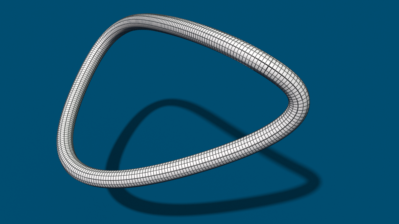
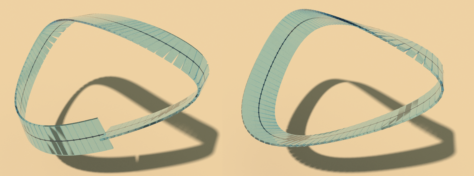
One possible application of frames is to draw a tubular surface around a given curve: Let $\gamma$ is a closed discrete curve and $\psi$ a frame of $\gamma$. Then the $\epsilon$-tube can be parametrized by$$f:{\mathfrak{S}}_n^1\times {\mathfrak{S}}_m^1\to {\mathbb{R}}^3,(j,k)\mapsto {\gamma }_j+\epsilon {\psi }_j{e}^{\pi \mathbf{i}k/m}\mathbf{j}{e}^{-\pi \mathbf{i}k/m}\overline{{\psi }_j}.$$ This we can use to create our own improved version of the polywire node.

Homework (due 17/19 May): Create a tubular surface node, i.e. write a network that computes for any given closed discrete curve a parametrized tube around it. To do so use a frame of minimal constant torsion to modify the point positions of a standard torus provided by Houdini’s torus node. In one direction the resolution of the torus has to be chosen to coincide with the number of points of the input curve. Make it possible to change the resolution in the other direction.

Hint: To set the number of columns of the torus one can use the Expression function npoints in the parameter field Columns of the Torus Node.